Design of IIR Filters: Signal Flow Graphs and Filter Implementations

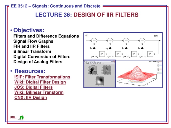
ECE 8443 Pattern Recognition EE 3512 Signals: Continuous and Discrete LECTURE 36: DESIGN OF IIR FILTERS Objectives: Filters and Difference Equations Signal Flow Graphs FIR and IIR Filters Bilinear Transform Digital Conversion of Filters Design of Analog Filters Resources: ISIP: Filter Transformations Wiki: Digital Filter Design JOS: Digital Filters Wiki: Bilinear Transform CNX: IIR Design URL:

Converting Difference Equations To Signal Flow Graphs Recall our expression for a linear, constant-coefficient difference equation: [ ... ] 2 [ ] 1 [ ] [ 2 1 n y a n y a n y a n y N + + + + = + ] 1 + + ] [ ] [ ... [ ] N b x n b x n b x n M 0 1 M This equation can be written succinctly using summations: = = l k 0 1 N M = + [ ] [ ] [ ] y n a y n k b x n l k l We can draw a signal flow graph implementation of this equation: 0b [n y ] [n x ] + + 1b 1a + + 1 1 z z 2b 2 a + + 1 1 z z . . . . . . This is known as the Direct Form I implementation of the above difference equation. Can we implement this more efficiently? EE 3512: Lecture 36, Slide 1

Direct Form II: Sharing Delay Elements (Memory) One of the more elementary aspects of the field of digital signal processing is to develop more efficient implementations of digital filters, as well as improve their ability to produce accurate results with less numerical precision. A more efficient implementation of our filter is a Direct Form II: + 0b [n y ] [n x ] + 1b 1a + + 1 z 2b 2 a + + 1 z . . . This filter has the same transfer function, but shares the delay element between the feedforward (moving average/finite impulse response) and feedback (autoregressive/infinite impulse response) portions of the filter. Analog differential equations can be represented by similar signal flow graphs, but their implementation involves physical components (e.g., RLCs, op amps). EE 3512: Lecture 36, Slide 2

More About Types of Filters Consider a filter with only feedforward components: The transfer function is: = l z Y z H ) ( M = [ ] [ ] y n b x n l l 1 ( ) M = l = = l ( ) b z l X z 0 Since the impulse response of this filter, h[n], has a finite number of nonzero terms, this filter is referred to as a finite impulse response (FIR) filter. Observe that this filter only has zeroes. Next, consider a filter with only feedback components: The transfer function is: = k b z H 1 N = + [ ] [ ] [ ] y n a y n k b x n 0 k 1 = 0 ( ) N = k + k a z k 1 This is an all-pole filter with an infinite impulse response (IIR). Why? EE 3512: Lecture 36, Slide 3

Design of Digital Filters Using Analog Prototypes Analog filter design theory was developed in the mid-1900 s. As digital signal processing developed, it seemed reasonable to leverage existing knowledge in analog filter design. Our strategy will be to design the filter in the analog domain, and then transform the filter to the digital domain. We can derive this transformation by recalling the relationship between the Laplace transform and the z-transform: 1 z T = = sT ln( ) z e s We can approximate the logarithm using a Taylor series: + + 1 1 T z T T 1 1 2 1 2 1 z z = = ln( ) s z 1 z This transformation is known as the bilinear transform. It maps the left-half s-plane to the interior of the unit circle in the z-plane. Unfortunately, it also warps the frequency axis, so the analog filter design must be prewarped so that it lands at the proper frequency in the z-plane. Let s = + j and z = re j : j 2 1 re + j = j + 1 T re EE 3512: Lecture 36, Slide 4

Frequency Warping In the Bilinear Transform We can solve for and by equating real and imaginary parts: 2 2 2 T 1 r r = + + 2 1 cos r cos r 2 T 2 2 sin r = + + 1 2 r To understand the implications on frequency response, set r = 1 and = 0 : 2 T sin 2 T = = tan + 1 cos 2 T = 1 2 tan 2 This suggests a design strategy where: (1) Establish requirements (e.g., cutoff frequency of c = 2 (1 kHz)/(8 kHz)). 2 T = (2) Prewarp by computing the equivalent analog frequency: . tan c c 2 (3) Design an analog filter, generating H(s). = ( ) ( ) H z H s (4) Derive: 2 T 1 z = s + 1 z EE 3512: Lecture 36, Slide 5

Design Example: Butterworth Lowpass Filter Recall our expression for a second-order Butterworth filter: 2 ) ( s s + + = c H s 2 2 c 2 c (1) Requirements: Let our sample frequency be 5 Hz, and our desired lowpass cutoff frequency be 0.318Hz (2 rd/sec). Our desired digital cutoff frequency is 2 rd/sec * (1/5 Hz) = 0.4 rd. 2 2 Hz f c c = = 2 = + + s s s c c 1 ( 0309 . 0 ) ( ) ( + z z T 2 T 4 . 0 (2) Prewarp: = = = tan tan . 2 027 / sec c rd ( / 1 ) c 5 2 / 2 . 0 323 shifted ( 16 . 0 from . 0 318 ) Hz (3) Derive: = ( ) c H s + + + 2 . 0 + 567 2 + . 0 z 16 ) z 2 2 s 2 (4) Derive: 1 2 z = = H z H s 2 1 z 1 2 = 1 . 1 444 5682 . 0 s 1 (5) Compare frequency responses: + + 1 2 0302 . 0 1 ( 2 ) z z = ( ) H z 4514 . 1 5724 . 0 + 1 2 1 no warping z z + + 1 2 0309 . 0 1 ( z 2 ) z z = ( ) H z . 1 5682 . 0 + 1 2 1 444 prewarped z EE 3512: Lecture 36, Slide 6

Design of Analog Filters in MATLAB Butterworth: Let our sample frequency be 5 Hz, and our desired lowpass cutoff frequency be 0.318Hz (2 rd/sec). Our desired digital cutoff frequency is 2 rd/sec * (1/5 Hz) = 0.4 rd. [z, p, k] = buttap(2); % creates a 2-pole filter [num, den] = zp2tf(z, p, k); wc = 2; % desired cutoff frequency [num, den] = lp2lp(num, den, wc); T = 0.2; [numd, dend] = bilinear(num, den, 1/T); numd = [0.0302 0.0605 0.5724] dend = [1 -1.4514 0.5724] Chebyshev Type 1 Highpass Filter: Let our sample frequency be 5 Hz, and our desired highpass cutoff frequency be 0.318Hz (2 rd/sec). Our passband ripple is 3 dB. N = 2; % number of poles; Rp = 3; % passband ripple; T = 0.2; % sampling period; wc = 2; % analog cutoff frequency; Wc = wc * T / pi; % normalized cutoff frequency [numd, dend] = cheby1(N,Rp,Wc, high ); numd = [0.5697 -1.1394 0.5697] dend = [1 -1.516 0.7028] Note that a direct digital design can be done using the butter command. Note this filter was designed directly in the digital domain. EE 3512: Lecture 36, Slide 7

Summary Introduced realizations of difference equations using signal flow graphs. Introduced the concept of FIR and IIR filters. Discussed a method for transforming an analog filter to a digital filter that preserves the stability of the filter. Described a method to prewarp the frequency axis so that the analog filter results in a digital filter at the correct frequency. Demonstrated this design process using Butterworth and Chebyshev prototype analog filters. EE 3512: Lecture 36, Slide 8