Differential Equation Methods and Stability Analysis

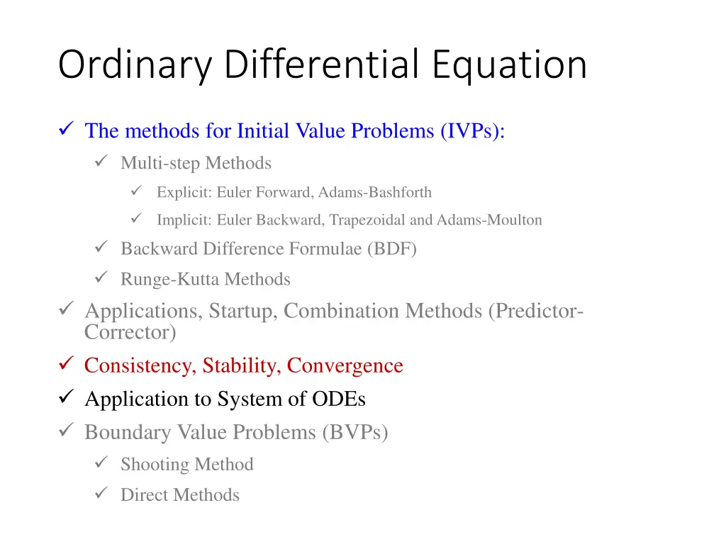
Ordinary Differential Equation The methods for Initial Value Problems (IVPs): Multi-step Methods Explicit: Euler Forward, Adams-Bashforth Implicit: Euler Backward, Trapezoidal and Adams-Moulton Backward Difference Formulae (BDF) Runge-Kutta Methods Applications, Startup, Combination Methods (Predictor- Corrector) Consistency, Stability, Convergence Application to System of ODEs Boundary Value Problems (BVPs) Shooting Method Direct Methods

Applications: Summary of Concerns Accuracy of the higher order multi-step and BDF methods are affected if the starting values are used from the lower order methods. How to start these non-self starting algorithms? All implicit methods (multi-step and BDF) may involve solution of non-linear equations (if f contains a non-linear function of the dependent variable y) Is there a way to avoid this solution of non-linear equations? Numerical oscillations (instability) observed in some methods and not in some! Is there a way to predict and therefore, choose correct parameters for algorithm so that the numerical oscillations can be avoided? We will do Convergence Analysis!

ODE: Consistency, Stability, Convergence (Recap; Text Book S6.3.2) A consistent numerical method is said to have an order of accuracy of p, if p is the largest positive integer such that ??? ? ?for 0 < ?, where K and h are constants. For all the methods derived so far, p 1, therefore, consistent! If numerical solutions for an IVP are obtained using a method with two sets of initial conditions ?0,?1,?2, ?? ?0,?1,?2, ?? , the method is stable if there exists a constant K such that the following relation holds as h 0, ??+m ??+m ? max ?0 ?0, ?1 ?1, ?? ?? Zero stability defines stability in asymptotic limit h 0 and ? Consistency and zero stability are necessary conditions for convergence

Numerical Methods for IVPs: Stability For application with h > 0, let us define an amplification factor ( ) ??+1 ?? = ? can be real or complex Condition of stability is satisfied if ? < 1 We need a model problem to assess and compare stability of various methods!

Stability: Model Problem Mathematical Problem: ?? ??= ? ?,? ? ?0 = ?0 ? 0 Using Taylor series expansion in the neighbourhood of fixed initial point (y0, t0) : 2 ?2? ??2 ?? ??= ? ?0,?0 + ? ?0 ?? ?? ?? ?? ? ?0 2 + ? ?0 + ?0,?0 ?0,?0 ?0,?0 ?2? ???? 2 ?2? ??2 ? ?0 2 + ? ?0 ? ?0 + + ?0,?0 ?0,?0 Collecting only the linear terms: ?? ??= ? + ?? + ?? + ?? ??= ?? + ? ?

Stability: Model Problem ?? ??= ?? + ? ? Any approximate solution ? computed using a numerical method satisfies the approximate equation ? ? ??= ? ? + ? ? The error ( ) is defined as: ? = ? ?. We may write: ?? ??= ?? The function of the independent variable ? ? has no influence on the progression of error in the equation. Therefore the model problem for linear stability analysis is: ?? ??= ??; We may evaluate the analytical solution in a discrete grid ?0,?1,?2, ?? with a time step of h: ??= ?0??? ? = ?0??? ? 0 = ?0

Stability: Model Problem For general applicability to all types of functions or problems, we let to be complex: ? = ??+ ??? ??= ?0??? = ?0??? ??? ?? ? The analytical solution grows unbounded, i.e., ? > 1 if ?? > 0 irrespective of the value of ?? ?? We will now derive the stability regions of the numerical methods in the ?? vs. ?? - plane and compare that with the stability region of the analytical solution. ?? Stability region of the analytical solution of the model problem in the ?? vs. ?? - plane

Stability: Multi-Step Methods (explicit) Example Recall: The stability region (in the ?? vs. ?? - plane) of a numerical method is an open set C that contains the collection of those h for which ? < 1. Boundary of the region is often characterized by ? = 1. Since, is a function of h, is complex: ? = ??? ???= 1 ? < 1 < 1 Euler Forward: applying the method to the model problem, ?? ??= ??; ? 0 = ?0 ??= ???0 ??+1= ??+ ? ??= 1 + ?? + ??? ??= ??? 1 + ?? 2+ ?? 2< 1 ? = 1 + ?? + ??? < 1 For real : ??= 0; ??= ? (necessary for stability) 0 < <2 ?

Stability: Multi-Step Methods (explicit) Example Consider our problem: ?? ??= 2? + sin? For stability with Euler forward, h < 1 0 < <2 ?

Stability: Multi-Step Methods (explicit) Example For higher order methods, let s consider 3rd order Adams-Bashforth: Adams-Bashforth (3rd Order): applying the method to model problem: 23 12??? 4 5 12??? 2 ??+1= ??+ 3??? 1+ ?3 ?2 23 12?2 4 ? = ?? + ??? = 3? +5 12 ??+1 ?? = ?;??+1 ?? ?? 2= ?2; ?? 1 ?? 2= ? By recursively applying ?? 2= ?3; In order to plot the region, recall that the boundary of the region is characterized by ? = 1 or ? = ??? cos3? cos2? + ? sin3? sin2? 23 12cos2? 4 ?? + ??? = 3cos? +5 23 12sin2? 4 12+ ? 3sin? One can now easily compute ?? and ?? for ? 0,2? Let s compare the stability regions of all the explicit multi-step methods!

Stability: Multi-Step Methods (explicit) Example All explicit methods are conditionally stable. Consider our problem: ?? ??= 2? + sin? For stability with Adams-Bashforth (4th Order), h < 0.3/2 = 0.15

Stability: Multi-Step (Implicit) Euler Backward: applying the method to the model problem, ??+1 ?? 1 1 1 ??+1= ??+ ???+1 = ? = 1 ? = 1 ?? ??? = ?? 1 ?? ???? ? = tan 1 1 ?? 2+ ?? 2; ? = 1 ? 1 ?? 2+ ?? 2> 1 ? < 1 < 1 Euler Backward method is stable everywhere outside the circle! Homework: Stability region of the Trapezoidal Method!

Stability: Multi-Step Methods (implicit) Example For higher order methods, let s consider 3rd order Adams-Moulton: Adams-Moulton (3rd Order): applying the method to the model problem, 5 12???+1+2 1 12??? 1 ??+1= ??+ 3??? ?2 ? 3? 1 cos2? cos? + ? sin2? sin? 12cos2? +2 ?? + ??? = = 12?2+2 5 5 3cos? 1 12sin2? +2 5 12+ ? 3sin? 12 One can now easily compute ?? and ?? for ? 0,2? Let s compare the stability regions of all the implicit multi-step methods!

Stability: Multi-Step Methods (implicit) Example Euler backward method is unconditionally stable! (It is stable everywhere, where the analytical problem is also stable) Trapezoidal: find as homework! Adams-Moulton 3rd and 4th order methods are conditionally stable! Pay attention to the stability for purely imaginary !

Stability: BDF Methods Example 1storder BDF is the Euler Backward. For higher order methods, let s consider 3rd order BDF: BDF (3rd Order): applying the method to the model problem, 11 6??+1 3??+3 11 6 3 2?? 1 1 3 2?2 3?? 2= ? ??+1 1 ? = ?? + ??? = ?+ 3?3 ??+1 ?? = ?;??+1 ?? ?? 2= ?2; ?? 1 ?? 2= ? By recursively applying ?? 2= ?3; 11 6 3cos? +3 2cos2? 1 3cos3? ? 3sin? 3 2sin2? +1 = 3sin3? One can now easily compute ?? and ?? for ? 0,2? Let s compare the stability regions of all the BDF methods!

Stability: BDF Methods Example For all the BDFs: Stability Region is outside the enclosed region! For real , all the BDFs are unconditionally stable! One can use any h without having to worry about the stability! Useful for stiff equations!

Stability: Runge-Kutta Methods Example Let s consider 2nd order Runge-Kutta method for illustration: R-K Method (2nd Order): applying the method to the model problem, ??+1= ??+1 2?1, ?0= ? ??,??, ?1= ? ??+ ?0,??+ ??+1= ??+1 2 ? ??+ ??? 1 + ? +1 ?? One needs to find the roots of the polynomial to compute ?? and ?? for ? 0,2? 2?0+1 2 ???+1 2? 2=??+1 = ? = ???= cos? + ?sin?, ? 0, 2? For 2nd order R-K, the roots of the quadratic polynomial can be computed analytically! For the 3rd and 4th order R-K, the roots have to be computed numerically. Use complex version of Newton-Raphson. (Hint: roots are complex conjugates) Let s compare the stability regions of 2nd and 4th order R-K methods!

Stability: Runge-Kutta Methods Example 4th order R-K has very good stability properties ( h up to 2.78 on the real part and 2.83 on the imaginary part) The method is also stable for purely imaginary h Homework: For our problem, check the stability limits of the R-K methods!

Phase Error Let s consider a problem with purely imaginary : ?? ??= ???, Analytical Solution: ??= ?0??? ? = ?0cos? ? + ?sin? ? ? 0 = ?0 Let s apply Euler Forward: ??+1= ??1 + ?? Solve with ? = 1; ?0= 1 and = ?/10 For periodic functions, there are phase error associated with the numerical solution. Can we quantify them?

Phase Error Let s consider a problem with purely imaginary : ?? ??= ???, Analytical Solution: ??= ?0??? ?= ?0cos? ? + ?sin? ? The amplification factor is: ?????=??+1 ?? ?0??? ? ? 0 = ?0 =?0??? ?+1 = ??? Amplitude: |?????| = cos2? + sin2? = 1 sin? cos? Phase: ?????= tan 1 = ? We will compare the amplitude and phase of the amplification factor of the numerical methods!

Phase Error Euler Forward: ??+1= ??1 + ?? ? = 1 + ?? Amplitude: |?| = 1 + ? 2> |?????| = 1 (No surprise here! We already know that Euler Forward method is not stable for purely imaginary ) Im ? Re ? Phase: ? = tan 1 = tan 1? ? 5 5! ? 3 3! ? 7 7! ? 9 9! tan 1? = ? + + Phase Error (PE) for Euler Forward is given by, ? 3 3! ? 5 5! ? 7 7! ? 9 9! ?? = ????? ? = ? tan 1? = +

Phase Error Euler Backward: 1 1 ?? , ? = ? 3 6 1 1 + ? 2, ? = tan 1? ,?? = ? = Trapezoidal: 1 + ?1 1 ?1 2? ? 3 12 , |?| = 1, ? = 2tan 1? ? = ,?? = 2 2? Runge-Kutta (2nd Order): ? 2 2 ? 4 4 ? , ? = tan 1 ? = 1 + ?? , ? = 1 + 1 ? 2 2 ? 3 6 ?? = Positive PE: phase lag Negative PE: phase lead

Arbitrary f How to choose time step h for arbitrary non- linear f: Expand fin Taylor s series around the initial condition, retain the first two terms (linear terms) to obtain the equivalent model problem set = coefficient of y compute h from the stability diagram! To account for the non-linearity, stay well below the stability limit!