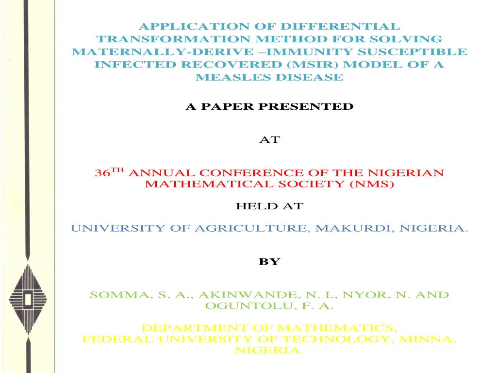
Differential Transformation Method for Measles Disease Model

APPLICATION OF DIFFERENTIAL TRANSFORMATION METHOD FOR SOLVING MATERNALLY-DERIVE IMMUNITY SUSCEPTIBLE INFECTED RECOVERED (MSIR) MODEL OF A MEASLES DISEASE A PAPER PRESENTED AT 36TH ANNUAL CONFERENCE OF THE NIGERIAN MATHEMATICAL SOCIETY (NMS) HELD AT UNIVERSITY OF AGRICULTURE, MAKURDI, NIGERIA. BY SOMMA, S. A., AKINWANDE, N. I., NYOR, N. AND OGUNTOLU, F. A. DEPARTMENT OF MATHEMATICS, FEDERAL UNIVERSITY OF TECHNOLOGY, MINNA, NIGERIA.

INTRODUCTION Measles is an airborne disease which spreads easily through the coughs and sneezes of those infected. It may also be spread through contact with saliva or nasal secretions. Nine out of ten people who are not immune and share living space with an infected person will likely catch it. People are infectious to others from four days before to four days after the start of the rash. People usually do not get the disease more than once in a life time; indicating that once recovered from the disease, the person become permanently immune (Atkinson, 2011).

INTRODUCTION CONTD According to WHO, measles is one of the leading causes of death among young children even though a safe and cost- effective vaccine is available. In 2015, there were 134 200 measles deaths globally about 367 deaths every day or 15 deaths every hour. Measles vaccination resulted in a 79% drop in measles deaths between 2000 and 2015 worldwide. In 2015, about 85% of the world's children receive xone dose of measles vaccine by their first birthday through routine health services up from 73% in 2000. During 2000-2015, measles vaccination prevented an estimated 20.3 million deaths making measles vaccine one of the best buys in public health.

INTRODUCTION CONTD Differential Transformation Method (DTM) is one of the method use to solve linear and nonlinear differential equations. It was first proposed by Zhou, (1986), for solving linear and nonlinear initial value problems in electrical circuit analysis. The DTM construct a semi-analytical numerical technique that uses Taylor series for the solution of differential equations in the form of a polynomial. DTM is a very effective and powerful tool for solving different kinds of differential equations. The main advantage of this method is that it can be applied directly to linear and nonlinear Ordinary Differential Equations (ODEs) without linearization, discretization or perturbation.

WHAT WE HAVE DONE In this paper: We used DTM to solve the MSIR model of the measles disease The DTM solution was validated with Runge-Kutta 4-5th order in Maple software The DTM solutions were presented graphically

MODEL EQUATIONS ( )M N + dM = (2.1) dt dS SI = ( + ) M v S (2.2) dt N dI SI = + + ( ) I (2.3) dt N dR = + I R vS (2.4) dt Where, N = + + + . R M S I

MODEL EQUATIONS CONTD Definition of Variables and Parameter of the Model M = passively immune infants S = Susceptible class I = Infected class R = Recovered class N = Total Population = Contact rate = recruitment rate = natural death rate = death rate due to disease = loss of temporal immunity period = recovery rate v= vaccination rate = Birth rate

SOLUTION OF THEMODEL Solution of the Model Equations using Differential Transformation Method (DTM) In this section we are going to apply Differential Transformation Method to the Model equation and solve. Let the model equation be a function ( ) t in Taylor series about a point = t , ( ) t h h can be expanded 0 as k k t d h ( ) t = k = h (2.4) k 0 ! k dt = 0 t Where, ( ) t h ) t = ( ), ( ), ( ), ( m t s t i t r (2.5)

SOLUTION OF THE MODEL CONTD The differential transformation of ( ) t h is defined as k 1 k d h ( ) t = H (2.6) k ! dt = 0 t Where, ( ) t H ) t = ( ), ( ), ( ), ( M t S t I t R (2.7) Then the inverse differential transform is ( ) t ( ) t = = k h t H (2.8) 0 k

SOLUTION OF THE MODEL CONTD Using the fundamental operations of differential transformation method, we obtain the following recurrence relation of equation (3.1) to (3.4) as 1 ( ) ( ) + = + 1 M k N M + 1 k 1 k ( ) ( ) ( m ) ( ) ( ) S = + = + 1 S k M S I k m v k + 1 k N 0 m 1 k ( ) ( ) ( m ) ( ) ( ) I = + = + + 1 I k S I k m k (2.9) + 1 1 k N 0 m ( ) + = + 1 I k I R vS + 1 k

SOLUTION OF THE MODEL CONTD With initial conditions ( ) 010 , 82 0 = M ( ) 0 ( ) 0 ( ) 118270718 0 = R (2.10) = = 000 , , , 7 099 , 464 364 , , 254 918 , , S I The parameter values are = = = = = = , 7 300 000 , = 000 , , . 0 005 , , 9 . 0 . 0 019 , . 0 53 , . 0 008 , N 1 = = . 0 85 , . 0 47 , . 0 39 v We consider We are going to considered three cases, varying different values of vaccination rate, v (2.11) = , 0 , 1 , 2 3 k

SOLUTION OF THE MODEL CONTD = . 0 85 v Case 1: Substituting (2.10) and (2.11) into (2.9) for ( ) ( ) ( ) ( ) ( ) ( ) ( ) ( ) = 159414975 4 R = , 0 , 1 , 2 3 k gives ( ) 2 ( ) 3 = = = 1 106060020 M , 48244056 , 3983255 , M M M = 4 30711621 ( ) 2 ( ) 3 = = = 1 6059579648 S , 262035140 , 743157523 , S S S = , 4 16327345 I ( ) 3 ( ) ( ) 3 = 6033718355 = = = 749350235 1 33834 2 92976 , 39990 , 4 7466 I I I ( ) 2 = = = 1 , 2599464175 , , R R R (2.12)

SOLUTION OF THE MODEL CONTD = , 0 , 1 , 2 3 k Substituting (2.12) into (2.8) for ( ) ( ) = = = 0 k gives + + + 2 3 k . t 82010000 106060020 48244056 3983255 m t m k t t t + 4 30711621 t ( ) t ( ) k = k = = + 2 3 k . t 7099464364 6059579648 262035140 74315752 s s t t t 0 + 4 16327345 t ( ) ( ) k = k = = + + 2 3 4 k . t 254918 33834 92976 39990 7466 t i i t t t t 0 ( ) t ( ) k = k = = + + 2 3 k . t 118270718 6033718355 2599464175 749350235 r r t t t 0 4 159414975 t (2.13)

SOLUTION OF THE MODEL CONTD = . 0 50 v Case 2: Substituting (2.10) and (2.11) into (2.9) for ( ) ( ) ( ) ( ) ( ) ( ) ( ) ( ) = 19186708 4 R = , 0 , 1 , 2 3 k gives ( ) 2 ( ) 3 = = = 1 106060020 M , 48244056 , 3983255 , M M M = 4 30711621 ( ) 2 ( ) 3 = = = 1 357476121 S , 928743534 , 150994477 , S S S = , 4 16327345 I ( ) 3 ( ) = = 3548905828 = = = 1 33834 2 53929 , 17085 , 4 3220 I I I ( ) 2 ( ) 3 = = 1 , 907895354 , 157203194 , R R R (2.14)

SOLUTION OF THE MODEL CONTD = , 0 , 1 , 2 3 k Substituting (2.14) into (2.8) for ( ) ( ) = = = 0 k gives + + + 2 3 k . t 82010000 106060020 48244056 3983255 m t m k t t t + 4 30711621 t ( ) t ( ) k = k = = + 2 3 k . t 7099464364 357476121 928743534 150994477 s s t t t 0 + 4 16327345 t ( ) ( ) k = k = = + + 2 3 4 k . t 2549918 33834 53929 17085 3220 t i i t t t t 0 ( ) t ( ) k = k = = + + 2 3 k . t 118270718 3548905828 907895354 157203194 r r t t t 0 4 19186708 t (2.15)

SOLUTION OF THE MODEL CONTD 25 . 0 = v Case 3: Substituting (2.10) and (2.11) into (2.9) for = , 0 , 1 , 2 3 k gives ( ) 1 ( ) 2 ( ) 3 = = = 106060020 M , 48244056 , 3983255 , M M M ( ) 4 = 30711621 ( ) 1 ( ) 2 ( ) 3 = = = 1799901030 S , 252912028 , 15476262 , S S S ( ) 4 = , 4879493 I ( ) ( ) 1 R ( ) 2 ( ) 3 ( ) 3 = 1774033973 R = R = = 21690834 1 33834 263039 , 6304 , 4 850 I I I ( ) 2 ( ) = = = , 7 232091739 , , R ( ) 4 = 1009907 (2.16)

SOLUTION OF THE MODEL CONTD = , 0 , 1 , 2 3 k Substituting (2.16) into (2.8) for ( ) ( ) = = = 0 k gives + + + 2 3 k . t 82010000 106060020 48244056 3983255 m t m k t t t + 4 30711621 t ( ) t ( ) k = k = = + 2 3 k . t 7099464364 1799901030 252912028 15476262 s s t t t 0 + 4879493 ( ) ( ) k = k = = + + 2 3 4 k . t 2549918 33834 263039 6304 850 t i i t t t t 0 ( ) t ( ) k = k = = + + 2 3 k . t 118270718 1774033973 7 232091739 21690834 r r t t t 0 4 1009907 t (2.17)

RESULTS AND DISCUSSION Numerical Solution of DTM and Runge-Kutta We compared the DTM solutions with the Runge-Kutta impeded in Maple software Table 1: Numerical solution of Maternally-Derived- Immunity t 0 0.1 0.2 105519568.4736 102399727.9392 0.3 119494224.9551 112001868.6768 0.4 135488583.5776 21229349.5002 0.5 153999619.6875 130096788.8131 0.6 175598016.5216 138618235.0603 0.7 200928165.2071 146807188.2767 0.8 230708164.7616 154676621.6537 0.9 265729822.0931 162239002.6453 1.0 306858652.0000 169506311.5421 DTM RUNGE-KUTTA 82010000.0000 82010000.0000 93141346.6771 92407714.9923

RESULTS AND DISCUSSION CONTD Table 2: Numerical solution of Susceptible t 0 0.1 6518983083.0328 6518973604.2711 0.2 5986678467.7888 5986595001.9527 0.3 5498679357.5788 5498357705.5832 0.4 5051506448.0128 5050617796.2627 0.5 4642072291.0000 4640031884.8469 0.6 4267681294.7488 4263531508.1332 0.7 3926029723.7668 3918301369.1918 0.8 3615205698.8608 3601758125.8419 0.9 3333689197.1368 3311531021.7912 1.0 3080352052.0000 3045445194.6477 DTM RUNGE-KUTTA 7099464364.0000 7099464364.00000

RESULTS AND DISCUSSION CONTD Table 3: Numerical solution of Infected t 0 0.1 0.2 0.3 0.4 0.5 0.6 0.7 0.8 0.9 1.0 DTM 254918.0000 254918.0000 250645.5766 250645.5030 244764.0256 244760.7979 237540.1646 237516.1576 229258.7296 229160.7508 220222.3750 219933.2495 210751.6736 210056.2946 201185.1166 199732.8615 191879.1136 189144.0930 183207.9926 178448.3956 175564.0000 167781.5011 RUNGE-KUTTA

RESULTS AND DISCUSSION CONTD Table 4: Numerical solution of Recovered/Immune t 0 0.1 696381320.4875 696381424.3608 0.2 1226775559.9200 1226781149.5879 0.3 1713375643.7975 1713424746.6791 0.4 2159721183.6800 2159940743.3293 0.5 2568969195.1875 2569657728.8486 0.6 2943894098.0000 2945629940.3248 0.7 3286887715.8575 3290659005.3171 0.8 3599959276.5600 3607315135.0971 0.9 3884735411.9675 3897956474.5273 1.0 4142460158.0000 4164745776.5776 DTM RUNGE-KUTTA 118270718.0000 118270718.0000

RESULTS AND DISCUSSION CONTD Graphical Solution of the Differential Transformation Solution Figure 1: The Population against time of High Vaccination rate

RESULTS AND DISCUSSION CONTD Figure 2: The Population against time of High Moderate Vaccination rate

RESULTS AND DISCUSSION CONTD Figure 3: The Population against time of Low Vaccination rate

CONCLUSION The method of solution gives us better understanding of the model. Immunization plays a vital role in preventing the outbreak of disease in the population. Attention should be given to immunization in order eradicate measles from the population. The numerical solutions shows that the Differential Transformation Method is in agreement with the Runge-Kutta.

THANK YOU FOR LISTENING