Digital Filter Design Techniques and Specifications

UNIT-IV FIR & IIR FILTERS

IIR filters 2

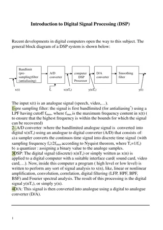
Filter Design Techniques Any discrete-time system that modifies certain frequencies Frequency-selective filters pass only certain frequencies Filter Design Steps Specification Problem or application specific Approximation of specification with a discrete-time system Our focus is to go from spec to discrete-time system Implementation Realization of discrete-time systems depends on target technology We already studied the use of discrete-time systems to implement a continuous-time system If our specifications are given in continuous time we can use n n y x xc(t) yr(t) H(ej ) D/C C/D ( ) ( ) j H e = H j / T c 3

Digital Filter Specifications Only the magnitude approximation problem Four basic types of ideal filters with magnitude responses as shown below (Piecewise flat) 4

Digital Filter Specifications These filters are unealisable because (one of the following is sufficient) their impulse responses infinitely long non- causal Their amplitude responses cannot be equal to a constant over a band of frequencies Another perspective that provides some understanding can be obtained by looking at the ideal amplitude squared. 5

Digital Filter Specifications The realisable squared amplitude response transfer function (and its differential) is continuous in Such functions if IIR can be infinite at point but around that point cannot be zero. if FIR cannot be infinite anywhere. Hence previous differential of ideal response is unrealisable 6

Digital Filter Specifications For example the magnitude response of a digital lowpass filter may be given as indicated below 7

Digital Filter Specifications In the passband we require that with a deviation 1 ) ( G 1 ) ( 1 0 p je p j + , G e p p p s In the stopband we require that with a deviation 0 ) ( e G s j je ( ) , G s s 8

Digital Filter Specifications Filter specification parameters - passband edge frequency - stopband edge frequency - peak ripple value in the passband - peak ripple value in the stopband p s p s 9

Digital Filter Specifications Practical specifications are often given in terms of loss function (in dB) Peak passband ripple Minimum stopband attenuation log 20 s = je = G ( ) 20 log ( ) G 10 = 20 log 1 ( ) dB 10 p p dB ( 10 ) s 10

Digital Filter Specifications In practice, passband edge frequency and stopband edge frequency are specified in Hz For digital filter design, normalized bandedge frequencies need to be computed from specifications in Hz using p F sF 2 F p p = = = 2 F T p p F F T T 2 F = = = 2 s s F T s s F F 11 T T

Digital Filter Specifications Example - Let kHz, kHz, and Then 10 25 10 25 = = 3 7 s F F p kHz = 25 T F 3 2 7 ( 10 ) = = . 0 56 p 3 3 2 3 ( 10 ) = = . 0 24 s 3 12

IIR Digital Filter Design Standard approach (1) Convert the digital filter specifications into an analogue prototype lowpass filter specifications (2) Determine the analogue lowpass filter transfer function (3) Transform by replacing the complex variable to the digital transfer function ) (z G (s ) Ha ) (s Ha 13

IIR Digital Filter Design This approach has been widely used for the following reasons: (1) Analogue approximation techniques are highly advanced (2) They usually yield closed-form solutions (3) Extensive tables are available for analogue filter design (4) Very often applications require digital simulation of analogue systems 14

IIR Digital Filter Design Let an analogue transfer function be ( ) P s = a ( ) H s a ( ) D s where the subscript a indicates the analogue domain A digital transfer function derived from this is denoted as ) ( D a ( ) P z = G z ( ) z 15

IIR Digital Filter Design (z ) G (s ) Ha Basic idea behind the conversion of into is to apply a mapping from the s-domain to the z- domain so that essential properties of the analogue frequency response are preserved Thus mapping function should be such that Imaginary ( ) axis in the s-plane be mapped onto the unit circle of the z-plane A stable analogue transfer function be mapped into a stable digital transfer function j 16

Specification for effective frequency response of a continuous-time lowpass filter and its corresponding specifications for discrete-time system. dp or d1 passband ripple ds or d2 stopband ripple Wp, wp passband edge frequency Ws, ws stopband edge frequency e2 passband ripple parameter 1 dp = 1/ 1 + e2 BW bandwidth = wu wl wc 3-dB cutoff frequency wu, wl upper and lower 3-dB cutoff frequensies Dw transition band = |wp ws| Ap passband ripple in dB = 20log10(1 dp) As stopband attenuation in dB = -20log10(ds) 17

Design of Discrete-Time IIR Filters From Analog (Continuous-Time) Filters Approximation of Derivatives Impulse Invariance the Bilinear Transformation 18

Reasons of Design of Discrete-Time IIR Filters from Continuous-Time Filters The art of continuous-time IIR filter design is highly advanced and, since useful results can be achieved, it is advantageous to use the design procedures already developed for continuous-time filters. Many useful continuous-time IIR design methods have relatively simple closed-form design formulas. Therefore, discrete-time IIR filter design methods based on such standard continuous-time design formulas are rather simple to carry out. The standard approximation methods that work well for continuous- time IIR filters do not lead to simple closed-form design formulas when these methods are applied directly to the discrete-time IIR case. 19

Characteristics of Commonly Used Analog Filters Butterworth Filter Chebyshev Filter Chebyshev Type I Chebyshev Type II of Inverse Chebyshev Filter 20

Butterworth Filter Lowpass Butterworth filters are all-pole filters characterized by the magnitude-squared frequency response |H(W)|2 = 1/[1 + (W/Wc)2N] = 1/[1 + e2(W/Wp)2N] where N is the order of the filter, Wc is its 3-dB frequency (cutoff frequency), Wp is the bandpass edge frequency, and 1/(1 + e2) is the band-edge value of |H(W)|2. At W = Ws (where Ws is the stopband edge frequency) we have 1/[1 + e2(Ws/Wp)2N] = d22 and N = (1/2)log10[(1/d22) 1]/log10(Ws/Wc) = log10(d/e)/log10(Ws/Wp) where d2= 1/ 1 + d22. Thus the Butterworth filter is completely characterized by the parameters N, d2, e, and the ratio Ws/Wp. 21

Butterworth Lowpass Filters Passband is designed to be maximally flat The magnitude-squared function is of the form ( ) ( ) c j / j 1 + 1 1 ( ) s 2 2 H j = H = ( ) c c 2 N 2 N 1 + s / j c ( ) ( ) ( )( ) 1 / 2 N j / 2 N 2 k + N 1 s = 1 j = e for k = 0,1,...,2N - 1 k c c 22

Frequency response of lowpass Butterworth filters 23

Chebyshev Filters The magnitude squared response of the analog lowpass Type I Chebyshev filter of Nth order is given by: where TN(W) is the Chebyshev polynomial of order N: TN(W) = cos(Ncos-1 W), |W| 1, = cosh(Ncosh-1 W), |H(W)|2 = 1/[1 + e2TN2(W/Wp)]. |W| > 1. The polynomial can be derived via a recurrence relation given by Tr(W) = 2WTr-1(W) Tr-2(W), with T0(W) = 1 and T1(W) = W. r 2, The magnitude squared response of the analog lowpass Type II or inverse Chebyshev filter of Nth order is given by: |H(W)|2 = 1/[1 + e2{TN(Ws/Wp)/ TN(Ws/W)}2]. 24

Chebyshev Filters Equiripple in the passband and monotonic in the stopband Or equiripple in the stopband and monotonic in the passband ( ) ( / V 1 N + ( ) 1 2 ( ) x 2 1 H j = V = cos N cos x ) c N 2 c 25

Frequency response of lowpass Type I Chebyshev filter |H(W)|2 = 1/[1 + e2TN2(W/Wp)] Frequency response of lowpass Type II Chebyshev filter |H(W)|2 = 1/[1 + e2{TN2(Ws/Wp)/TN2(Ws/W)}] 26

N = log10[( 1 - d22 + 1 d22(1 + e2))/ed2]/log10[(Ws/Wp) + (Ws/Wp)2 1 ] = [cosh-1(d/e)]/[cosh-1(Ws/Wp)] for both Type I and II Chebyshev filters, and where d2 = 1/ 1 + d2. The poles of a Type I Chebyshev filter lie on an ellipse in the s-plane with major axis r1 = Wp{(b2 + 1)/2b] and minor axis r1 = Wp{(b2 - 1)/2b] where b is related to e according to b = {[ 1 + e2 + 1]/e}1/N The zeros of a Type II Chebyshev filter are located on the imaginary axis. 27

Type I: pole positions are xk = r2cosfk yk = r1sinfk fk = [p/2] + [(2k + 1)p/2N] r1 = Wp[b2 + 1]/2b r2 = Wp[b2 1]/2b b = {[ 1 + e2 + 1]/e}1/N Type II: zero positions are sk = jWs/sinfk and pole positions are vk = Wsxk/ xk2 + yk2 wk = Wsyk/ xk2 + yk2 b = {[1 + 1 d22 ]/d2}1/N Determination of the pole locations for a Chebyshev filter. k = 0, 1, , N-1. 28

Approximation of Derivative Method Approximation of derivative method is the simplest one for converting an analog filter into a digital filter by approximating the differential equation by an equivalent difference equation. For the derivative dy(t)/dt at time t = nT, we substitute the backward difference [y(nT) y(nT T)]/T. Thus ] 1 ( ) ( ) ( ) [ ] [ dy t y nT y nT T y n y n = dt T T = t nT where T represents the sampling period. Then, s = (1 z-1)/T The second derivative d2y(t)/dt2 is derived into second difference as follow: ] 1 + ( ) [ ] 2 [ [ ] 2 dy t y n y n y n 2 dt T = t nT which s2 = [(1 z-1)/T]2. So, for the kth derivative of y(t), sk = [(1 z-1)/T]k. 29

Approximation of Derivative Method Hence, the system function for the digital IIR filter obtained as a result of the approximation of the derivatives by finite difference is H(z) = Ha(s)|s=(z-1)/Tz It is clear that points in the LHP of the s-plane are mapped into the corresponding points inside the unit circle in the z-plane and points in the RHP of the s-plane are mapped into points outside this circle. Consequently, a stable analog filter is transformed into a stable digital filter due to this mapping property. jW Unit circle s s-plane z-plane 30

Example: Approximation of derivative method Convert the analog bandpass filter with system function Ha(s) = 1/[(s + 0.1)2 + 9] Into a digital IIR filter by use of the backward difference for the derivative. Substitute for s = (1 z-1)/T into Ha(s) yields H(z) = 1/[((1 z-1)/T) + 0.1)2 + 9] 2 T = 2 2 . 0 + . 9 + ( ) H z 1 01 T T 1 . 0 + T + 1 2 1 ( 2 ) T 1 z z 1 2 2 2 . 0 + . 9 + 2 . 0 + . 9 + 1 01 1 01 T T T T can be selected to satisfied specification of designed filter. For example, if T = 0.1, the poles are located at p1,2 = 0.91 j0.27 = 0.949exp[ j16.5o] 31

Filter Design by Impulse Invariance Remember impulse invariance Mapping a continuous-time impulse response to discrete-time Mapping a continuous-time frequency response to discrete-time d T n h = ( = ( ) h nT c d ) T 2 j H e = H j + j k If the continuous-time filter is bandlimited to c T k d d ( ) H j = 0 / T c d If we start from discrete-time specifications Td cancels out Start with discrete-time spec in terms of Go to continuous-time = /T and design continuous-time filter Use impulse invariance to map it back to discrete-time = T Works best for bandlimited filters due to possible aliasing ( ) T j H e = H j c d 32

Impulse Invariance of System Functions Develop impulse invariance relation between system functions Partial fraction expansion of transfer function A N ( ) H s = k c s s k = 1 k Corresponding impulse response N = s t A e t 0 ( ) t k h k c k = 1 0 t 0 Impulse response of discrete-time filter ( ) u N N n n ( ) n = k = k s nT s T h = T h nT = T A e u = T A e n System function k d k d d c d d k d k 1 1 T A N ( ) H z = d k s T 1 1 e z s Pole s=sk in s-domain transform into pole at k d k = 1 kT e d 33

Impulse Invariant Algorithm Step 1: define specifications of filter Ripple in frequency bands Critical frequencies: passband edge, stopband edge, and/or cutoff frequencies. Filter band type: lowpass, highpass, bandpass, bandstop. Step 2: linear transform critical frequencies as follow W = w/Td Step 3: select filter structure type and its order: Bessel, Butterworth, Chebyshev type I, Chebyshev type II or inverse Chebyshev, elliptic. Step 4: convert Ha(s) to H(z) using linear transform in step 2. Step 5: verify the result. If it does not meet requirement, return to step 3. 34

Example: Impulse invariant method Convert the analog filter with system function Ha(s) = [s + 0.1]/[(s + 0.1)2 + 9] into a digital IIR filter by means of the impulse invariance method. The analog filter has a zero at s = - 0.1 and a pair of complex conjugate poles at pk = - 0.1 j3. Thus, ( ) 3 1 . 0 j s + 1 1 = + Ha s 2 2 1 . 0 + + 3 s j 1 1 ( ) z Then = + H 2 T 2 1 . 0 1 . 0 3 1 3 1 j T T j T 1 1 e e z e e z 35

Frequency response of digital filter. Frequency response of analog filter. 36

Disadvantage of previous techniques: frequency warping aliasing effect and error in specifications of designed filter (frequencies) So, prewarping of frequency is considered. 37

Example Impulse invariance applied to Butterworth 89125 . 0 ( ( ) ) j H e 1 0 0 . 2 j H e 0.17783 0 . 3 Since sampling rate Td cancels out we can assume Td=1 Map spec to continuous time ( ( ) ) 0 89125 . H j 1 0 0 . 2 H j 0.17783 0 . 3 Butterworth filter is monotonic so spec will be satisfied if ( ) 89125 . 0 2 . 0 j H c ( ) c j H ( ) and H 1 0 j . 3 0.17783 c 2 = ( ) 2 N 1 + j / j c Determine N and c to satisfy these conditions 38

Example Contd Satisfy both constrains 2 . 0 1 2 N 2 N 2 2 1 0 . 3 1 + = and 1 + = 0 89125 . 0 17783 . c c Solve these equations to get N = 5 8858 . 6 and c= 0 70474 . N must be an integer so we round it up to meet the spec Poles of transfer function ( ) ( ) j 1 s c k = = ( )( ) 1 / 12 j / 12 2 k + 11 e for k = 0,1,...,11 c The transfer function ( ) ( 364 . 0 s + 0 12093 . H s = )( )( ) 2 2 2 s + 0 4945 . s + 0 9945 . s + 0 4945 . s + 1 3585 . s + 0 4945 . Mapping to z-domain 1 1 0 2871 . 0 4466 . + z 2 1428 . + 1 1455 . + z ( ) z H = + 1 2 1 2 1 1 2971 . z 0 6949 . z 1 1 0691 . z 0 3699 . z 1 1 8557 . 0 6303 . + z + 1 2 1 0 9972 . z 0 257 . z 39

Example Contd 40

Filter Design by Bilinear Transformation Get around the aliasing problem of impulse invariance Map the entire s-plane onto the unit-circle in the z-plane Nonlinear transformation Frequency response subject to warping Bilinear transformation 1 2 1 z s = Transformed system function 1 T 1 + z d 1 2 1 z Again Td cancels out so we can ignore it We can solve the transformation for z as ( ) z H = H c 1 T 1 + z d Maps the left-half s-plane into the inside of the unit-circle in z Stable in one domain would stay in the other ( ) ( ) 1 s 2 / T 1 d 1 + T / 2 s 1 + T / 2 + j T / 2 s = + j z = = d d d T / 2 j T / 2 d d 41

Bilinear Transformation On the unit circle the transform becomes + = 1 1 j T / 2 j z = e d j T / 2 d To derive the relation between and + e 1 T d ( ( ) ) j j / 2 2 1 e 2 2 e j sin / 2 2 j 2 s = = + j = = tan j j / 2 T T 2 e cos / 2 d d Which yields T 2 2 = tan or = 2 arctan d T 2 d 42

Bilinear Transformation 43

Example Bilinear transform applied to Butterworth 89125 . 0 ( ( ) ) j H e 1 0 0 . 2 j H e 0.17783 0 . 3 Apply bilinear transformation to specifications ( j H 89125 . 0 2 0 . 2 ) 1 0 tan T 2 d 2 0 . 3 ( ) H j 0.17783 tan T 2 d We can assume Td=1 and apply the specifications to 1 ( ) 2 H j = ( ) c 2 N 1 + / To get c 2 N 2 N 2 2 2 tan 0 . 1 1 2 tan 0 15 . 1 1 + = and 1 + = 0 89125 . 0 17783 . c c 44

Example Contd Solve N and c 2 2 1 1 log 1 1 0 17783 . 0 89125 . c= 0 766 . N = = 5 305 . 6 ( ) ( ) 2 log tan 0 15 . tan 0 . 1 The resulting transfer function has the following poles ( ) ( ) e j 1 s c c k = = ( )( ) 1 / 12 j / 12 2 k + 11 for k = 0,1,...,11 Resulting in ( ) ( s + 0 20238 . H s = )( )( ) c 2 2 2 0 3996 . s + 0 5871 . s + 1 0836 . s + 0 5871 . s + 1 4802 . s + 0 5871 . Applying the bilinear transform yields ( 1 ) 6 1 0 0007378 . + z ( ) z H = ( 1 )( ) 1 2 1 2 1 2686 . z + 0 7051 . z 1 1 0106 . z + 0 3583 . z 1 ( 1 ) 1 2 0 9044 . z + 0 2155 . z 45

Example Contd 46

IIR Digital Filter: The bilinear transformation To obtain G(z) replace s by f(z) in H(s) Start with requirements on G(z) G(z) Available H(s) Stable Stable Real and Rational in z Real and Rational in s Order n Order n L.P. (lowpass) cutoff L.P. cutoff T c c 47

Bilinear Transformation Mapping of s-plane into the z-plane 48

Bilinear Transformation For with unity scalar we have 1 e + je z = j e = = tan( ) 2 / j j j 1 = tan( or ) 2 / 49

Bilinear Transformation Mapping is highly nonlinear Complete negative imaginary axis in the s- plane from to the lower half of the unit circle in the z-plane from to Complete positive imaginary axis in the s- plane from to is mapped into the upper half of the unit circle in the z-plane from to 1 = z 1 = z = is mapped into 0 = = = 1 z 1 z = = 0 50