Digital Signal Processing Applications and Techniques
Explore the world of Digital Signal Processing (DSP) through applications like audio processing, echo location, and pattern recognition. Learn how DSP is utilized in speech recognition, radar systems, and data classification. Discover the wide-ranging uses of DSP in various fields such as biometrics and Brain-Computer Interface (BCI).

Download Presentation

Please find below an Image/Link to download the presentation.
The content on the website is provided AS IS for your information and personal use only. It may not be sold, licensed, or shared on other websites without obtaining consent from the author. If you encounter any issues during the download, it is possible that the publisher has removed the file from their server.
You are allowed to download the files provided on this website for personal or commercial use, subject to the condition that they are used lawfully. All files are the property of their respective owners.
The content on the website is provided AS IS for your information and personal use only. It may not be sold, licensed, or shared on other websites without obtaining consent from the author.
E N D
Presentation Transcript
CSE 447 : Digital Signal Processing Dr. Md. SujanAli Associate Professor Dept. of Computer Science and Engineering Jatiya Kabi Kazi Nazrul Islam University
Reference Books Digital Signal Processing, fourth edition - John G. Proakis Digital Signal Processing, third edition - P. Ramesh Babu CSE 447, Digital Signal Processing, Dept. of Computer Science and Engineering April 12, 2025 2
Introduction to signals CSE 447, Digital Signal Processing, Dept. of Computer Science and Engineering April 12, 2025 3
- CSE 447, Digital Signal Processing, Dept. of Computer Science and Engineering April 12, 2025 4
Applications Digital Signal Processing (DSP) is being used very widely in applications that include- Audio signal processing/Speech recognition Eco location Pattern recognition Biometrics Brain Computer Interface (BCI) CSE 447, Digital Signal Processing, Dept. of Computer Science and Engineering April 12, 2025 5
DSP Application: Audio Processing o Audio signal processing/Speech recognition Speech recognition: DSP generally approaches the problem of voice recognition in two steps: feature extraction followed by feature matching. Source: Canon CSE 447, Digital Signal Processing, Dept. of Computer Science and Engineering 6 April 12, 2025
DSP Application: Echo Location A common method of obtaining information about a remote object is to bounce a wave off of it. Applications include radar and sonar. DSP can be used for filtering and compressing the data. Source: WHIO Source: CCTT.org CSE 447, Digital Signal Processing, Dept. of Computer Science and Engineering 7 April 12, 2025
DSP Application: Pattern Recognition Pattern recognition is a research area that is closely related to digital signal processing. Definition: the act of taking in raw data and taking an action based on the category of the data . Pattern recognition classifies data based on either a priori knowledge or on statistical information extracted from the patterns. Source: merl.com CSE 447, Digital Signal Processing, Dept. of Computer Science and Engineering 8 April 12, 2025
DSP Application: Biometrics The Biometrics field focuses on methods for uniquely humans using one or more of their intrinsic physical or behavioural traits. Examples include using face, voice, fingerprints, iris, handwriting or the method of walking. identifying Source: BBC CSE 447, Digital Signal Processing, Dept. of Computer Science and Engineering 9 April 12, 2025
DSP Application: Brain computer interface A means for communication between a brain and a computer via measurements associated activity. No muscle involved movement). with brain motion (e.g., is eye CSE 447, Digital Signal Processing, Dept. of Computer Science and Engineering 10 April 12, 2025
Why signals should be processed? o Signals are carriers of information Useful and unwanted Extracting, enhancing, storing and transmitting the useful information o How signals are being processed? Analog Signal Processing vs. Digital Signal Processing CSE 447, Digital Signal Processing, Dept. of Computer Science and Engineering April 12, 2025 11
Digital Signal Processing (DSP) System CSE 447, Digital Signal Processing, Dept. of Computer Science and Engineering April 12, 2025 12
Signal Basics Signals A signal is a function that represents the variation of a physical quantity with respect to any parameter (independent quantity e.g., time, distance, space, temperature etc.) which conveys information. Signal = f(t) = sin ( t) X axis used for independent quantity Y axis used for dependent quantity CSE 447, Digital Signal Processing, Dept. of Computer Science and Engineering April 12, 2025 13
Signal Basics Function A function is a relation between a set of inputs and a set of outputs. A function relates an input to an output. It is like a machine that has an input and an output. And the output is related somehow to the input. f(x)=x2 (we say f of x equals x squared) Function without name: y = x2 x= input, y=output, squaring is the relation CSE 447, Digital Signal Processing, Dept. of Computer Science and Engineering April 12, 2025 14
Examples of Signals Signals are everywhere and may reflect countless measurements of some physical quantity such as: electric voltages brain signals heart rates temperatures image luminance investment prices vehicle speeds seismic activity human speech CSE 447, Digital Signal Processing, Dept. of Computer Science and Engineering 15 April 12, 2025
Advantage of Digital Over Analog Signal Processing o Digital signals can convey information with greater noise immunity, because each information component (byte etc) is determined by the presence or absence of a data bit (0 or one). Analog signals vary continuously and their value is affected by all levels of noise. o Enables transmission of signals over a long distance. o Transmission is at a higher rate and with a wider broadband width. o It is more secure. o It is also easier to translate human audio and video signals and other messages into machine language. CSE 447, Digital Signal Processing, Dept. of Computer Science and Engineering April 12, 2025 16
Signal Basics Continuous-time signals A signal x(t) is said to be a continuous-time signal if it is defined for all time t. Discrete-time signals Discrete-time signal is defined only at discrete instant of time. Thus, in this case, the independent variable has discrete values only. CSE 447, Digital Signal Processing, Dept. of Computer Science and Engineering April 12, 2025 17
Signal Basics o What?! CSE 447, Digital Signal Processing, Dept. of Computer Science and Engineering April 12, 2025 18
Continuous Time Signals In continuous time signals the independent variable is continuous, and they are defined for a continuum of values They take on values in the continuous interval (a, b), where a can be - and b can be the symbol t is used to denote the continuous time independent variable Example CSE 447, Digital Signal Processing, Dept. of Computer Science and Engineering April 12, 2025 19
Discrete Time Signal Discrete time signals are defined only at discrete times and for these signals the independent variable takes on only a discrete set of values The symbol n is used to denote the discrete time independent variable Example CSE 447, Digital Signal Processing, Dept. of Computer Science and Engineering April 12, 2025 20
Signal Basics Data Acquisition Data acquisition (DAQ) is the process of measuring an electrical or physical phenomenon such as voltage, current, temperature, pressure, or sound with a computer. A DAQ system consists of sensors, DAQ measurement hardware, and a computer with programmable software. CSE 447, Digital Signal Processing, Dept. of Computer Science and Engineering April 12, 2025 21
Signal Basics Sampling In signal processing, sampling is the reduction of a continuous-time signal to a discrete-time signal. A sample is a value or set of values at a point in time and/or space. CSE 447, Digital Signal Processing, Dept. of Computer Science and Engineering April 12, 2025 22
Signal Basics Sampling Theory The Sampling Theory states that a signal can be exactly reproduced if it is sampled at a frequency F, where F is greater than twice the maximum frequency in the signal Nyquist Rate In general, to preserve the full information in the signal, it is necessary to sample at twice the maximum frequency of the signal. This is known as the Nyquist rate. CSE 447, Digital Signal Processing, Dept. of Computer Science and Engineering April 12, 2025 23
Signal Basics Aliasing When the signal is converted back into a continuous time signal, it will exhibit a phenomenon called aliasing. Aliasing is the presence of unwanted components in the reconstructed signal. These components were not present when the original signal was sampled. CSE 447, Digital Signal Processing, Dept. of Computer Science and Engineering April 12, 2025 24
Sampling of Analog Signals X(n)= xa(t) = xa(nT)= xa(n/Fs) , - < n < Where, xa(t) is the analog signal x(n) is the discrete time signal CSE 447, Digital Signal Processing, Dept. of Computer Science and Engineering April 12, 2025 25
Sampling Example 1.4.2 1. Consider the signal xa(t)=3 cos 100 t (a) Determine the minimum sampling rate required to avoid aliasing. (b) Suppose that the signal is sampled at the rate Fs=200 Hz. What is the discrete-time signal obtained after sampling? (c) Suppose that the signal is sampled at the rate Fs=75 Hz. What is the discrete-time signal obtained after sampling? CSE 447, Digital Signal Processing, Dept. of Computer Science and Engineering April 12, 2025 26
Sampling Example 1.4.3 Consider the signal xa(t)=3 cos 50 t + 10 sin 300 t cos 100 t What is the Nyquist rate for this signal? CSE 447, Digital Signal Processing, Dept. of Computer Science and Engineering April 12, 2025 27
Sampling Example 1.4.4 Consider the signal xa(t)=3 cos 2000 t + 5 sin 6000 t + 10 cos 12000 t (a) What is the Nyquist rate for this signal? (b) Assume now that we sample this signal using a sampling rate Fs=5000 samples/s. What is the discrete-time signal obtained after sampling? (c) What is the analog signal ya(t) that we can reconstruct from the samples if we use ideal interpolation? CSE 447, Digital Signal Processing, Dept. of Computer Science and Engineering April 12, 2025 28
Signal Basics Quantization A sequence of samples like x[n] is not a digital signal because the sample values can take on a continuous range of values. In order to complete analog to digital conversion, each sample value is mapped to a discrete level in a process called quantization. Quantization is opposite to sampling. It is done on y axis. CSE 447, Digital Signal Processing, Dept. of Computer Science and Engineering April 12, 2025 29
Signal Basics Quantization In a B-bit quantizer, each quantization level is represented with B bits, so that the number of levels equals 2B CSE 447, Digital Signal Processing, Dept. of Computer Science and Engineering April 12, 2025 30
Signal Basics Quantization Error Quantization error is the difference between the analog signal and the closest available digital value at each sampling instant from the A/D converter. When you quantize a signal, you introduce an error which can be defined as q[n]=xq[n] x[n] where q[n] is the quantization error, x[n] the original signal, and xq[n] of the quantized signal. The higher the resolution of the A/D converter, the lower the quantization error and the smaller the quantization noise. CSE 447, Digital Signal Processing, Dept. of Computer Science and Engineering April 12, 2025 31
Discrete-Time Signals: Time-Domain Representation Signals represented as sequences of numbers, called samples Sample value of a typical signal or sequence denoted as x[n] with n being an integer in the range - n x[n] defined only for integer values of n and undefined for noninteger values of n Discrete-time signal represented by {x[n]} CSE 447, Digital Signal Processing, Dept. of Computer Science and Engineering April 12, 2025 32
Discrete-Time Signals: Time-Domain Representation Discrete-time signal may also be written as a sequence of numbers inside braces: {x[n]}={ ,-0.2,2.2,1.1,0.2,-3.7,2.9, } In the above, x[-1]= -0.2, x[0]=2.2, x[1]=1.1, etc. The arrow is placed under the sample at time index n = 0 CSE 447, Digital Signal Processing, Dept. of Computer Science and Engineering April 12, 2025 33
Discrete-Time Signals: Time-Domain Representation Graphical representation of a discrete-time signal with real-valued samples is as shown below: CSE 447, Digital Signal Processing, Dept. of Computer Science and Engineering April 12, 2025 34
Discrete-Time Signals: Time-Domain Representation In some applications, a discrete-time sequence {x[n]} may be generated by periodically sampling a continuous-time signal xa(t) at uniform intervals of time CSE 447, Digital Signal Processing, Dept. of Computer Science and Engineering April 12, 2025 35
Discrete-Time Signals: Time-Domain Representation Here, n-th sample is given by x[n]=xa(t)|t=nT=xa(nT), n= ,-2,-1,0,1, The spacing T between two consecutive samples is called the sampling interval or sampling period Reciprocal of sampling interval T, denoted as FT , is called the sampling frequency: 1 = FT T 1 = FT T CSE 447, Digital Signal Processing, Dept. of Computer Science and Engineering April 12, 2025 36
Discrete-Time Signals: Time-Domain Representation Unit of sampling frequency is cycles per second, or hertz (Hz) , if T is in seconds Whether or not the sequence {x[n]} has been obtained by sampling, the quantity x[n] is called the n-th sample of the sequence {x[n]} is a real sequence, if the n-th sample x[n] is real for all values of n Otherwise, {x[n]} is a complex sequence CSE 447, Digital Signal Processing, Dept. of Computer Science and Engineering April 12, 2025 37
Discrete-Time Signals: Time-Domain Representation A complex sequence {x[n]} can be written as {x[n]}={xre[n]}+j{xim[n]} where xre and xim are the real and imaginary parts of x[n] The complex conjugate sequence of {x[n]} is given by {x*[n]}={xre[n]}-j{xim[n]} Often the braces are ignored to denote a sequence if there is no ambiguity CSE 447, Digital Signal Processing, Dept. of Computer Science and Engineering April 12, 2025 38
Discrete-Time Signals: Time-Domain Representation Example - {x[n]}={cos0.25n} is a real sequence {y[n]}={ej0.3n} is a complex sequence We can write {y[n]}={cos0.3n + jsin0.3n} ={cos0.3n} + j{sin0.3n} where {yre[n]}={cos0.3n} {yim[n]}={sin0.3n} CSE 447, Digital Signal Processing, Dept. of Computer Science and Engineering April 12, 2025 39
Discrete-Time Signals: Time-Domain Representation Example {w[n]}={cos0.3n}- complex conjugate sequence of {y[n]}.That is, {w[n]}= {y*[n]} j{sin0.3n}={e-j0.3n} is the CSE 447, Digital Signal Processing, Dept. of Computer Science and Engineering April 12, 2025 40
Discrete-Time Signals: Time-Domain Representation Two types of discrete-time signals: - Sampled-data signals in which samples are continuous-valued - Digital signals in which samples are discrete-valued Signals in a practical digital signal processing system are digital signals obtained by quantizing the sample values either by rounding or truncation CSE 447, Digital Signal Processing, Dept. of Computer Science and Engineering April 12, 2025 41
Discrete-Time Signals: Time-Domain Representation Example Amplitude Amplitude Time,t Time,t Boxedcar signal Digital signal CSE 447, Digital Signal Processing, Dept. of Computer Science and Engineering April 12, 2025 42
Discrete-Time Signals: Time-Domain Representation A discrete-time signal may be a finite-length or an infinite-length sequence Finite-length (also called finite-duration or finite- extent) sequence is defined only for a finite time interval: N1 n N2 where - < N1 and N2 < with N1 N2 Length or duration ofthe above finite-length sequence is N= N2 - N1+ 1 CSE 447, Digital Signal Processing, Dept. of Computer Science and Engineering April 12, 2025 43
Discrete-Time Signals: Time-Domain Representation Example x[n]=n2, -3 n 4 is a finite-length sequence of length 4 -(-3)+1=8 y[n]=cos0.4n is an infinite-length sequence CSE 447, Digital Signal Processing, Dept. of Computer Science and Engineering April 12, 2025 44
Discrete-Time Signals: Time-Domain Representation A length- N sequence is often referred to as an N-point sequence The length of a finite-length sequence can be increased by zero-padding, i.e., by appending it with zeros CSE 447, Digital Signal Processing, Dept. of Computer Science and Engineering April 12, 2025 45
Discrete-Time Signals: Time-Domain Representation Example 5 n 8 2 , 3 4 n n = [ ] xe n , 0 is a finite-length sequence of length 12 obtained by zero-padding x[n] =n2, -3 n 4 with 4 zero-valued samples CSE 447, Digital Signal Processing, Dept. of Computer Science and Engineering April 12, 2025 46
Discrete-Time Signals: Time-Domain Representation A right-sided sequence x[n] has zero-valued samples for n < N1 A right-sided sequence If N1 0, a right-sided sequence is called a causal sequence CSE 447, Digital Signal Processing, Dept. of Computer Science and Engineering April 12, 2025 47
Discrete-Time Signals: Time-Domain Representation A left-sided sequence x[n] has zero-valued samples for n N2 N n 2 A left-sided sequence If N2 0, a left-sided sequence is called a anti-causal sequence CSE 447, Digital Signal Processing, Dept. of Computer Science and Engineering April 12, 2025 48
Operations on Sequences A single-input, single-output discrete-time system operates on a sequence, called the input sequence, according some prescribed rules and develops another sequence, called the output sequence, with more desirable properties Discrete-time system x[n] y[n] Output sequence Input sequence CSE 447, Digital Signal Processing, Dept. of Computer Science and Engineering April 12, 2025 49
Operations on Sequences For example, the input may be a signal corrupted with additive noise Discrete-time system is designed to generate an output by removing the noise component from the input In most cases, the operation defining a particular discrete-time system is composed of some basic operations CSE 447, Digital Signal Processing, Dept. of Computer Science and Engineering April 12, 2025 50


 System")