Dimensionality Reduction Analysis for Multivariate Data: Methods and Techniques

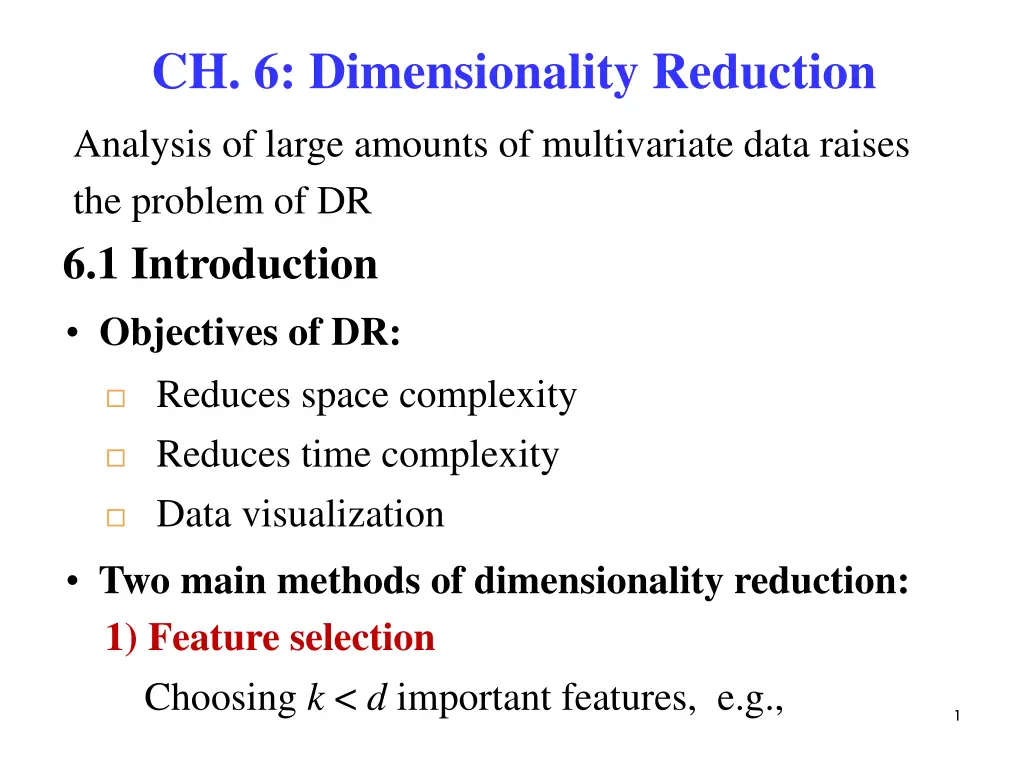
CH. 6: Dimensionality Reduction Analysis of large amounts of multivariate data raises the problem of DR 6.1 Introduction Objectives of DR: Reduces space complexity Reduces time complexity Data visualization Two main methods of dimensionality reduction: 1) Feature selection Choosing k < d important features, e.g., 1

Forward search, backward search, floating search 2) Feature extraction: Mapping data points from d-D to k-D space, where k < d, while preserving as many properties of the data as possible, e.g., Unsupervised extraction: principal component analysis, factor analysis, multidimensional scaling, canonical correlation analysis Supervised extraction: isometric feature mapping, locally linear embedding, Laplacian eigenmaps. 2

6.2 Feature Selection Forward search: Add the best feature at each step F = Initially, (F: feature set) At each iteration, find the best new feature using = a sample , where argmin ( i ) j E F x i E(): error function Add xj to F if ( ) ( ) E F E F x i Example: Iris data (3 classes: , 4 features: ) (F1,F2,F3,F4) 3

Single feature Accuracy 0.76 0.57 0.92 0.94 (chosen) 4

Add one more feature to F4 Accuracy 0.87 0.92 0.96 (chosen) Since the accuracies of (F1,F3,F4) and (F2,F3,F4) are both 0.94 smaller than 0.96. Stop the feature selection process at (F3,F4) . 5

Backward search: Start with all features and remove one at a time. j = argmin ( { }) i x E F Remove xjfrom F if i Floating search: The numbers of added and removed features can change at each step. 6

6.3 Feature Extraction 6.3.1 Principal Components Analysis (PCA) -- Linearly transforms a number of correlated features into the same number of uncorrelated features. ij = correlation coefficient ( , ) . x x Recall that i j i j = = = 0 Cov( , ) 0. x x Uncorrelation: ij i j Graphically, and axes are orthogonal. i j x x Independence: = ( , P x x ) ( ) ( ). i P x P x i j j 7

= = T x ( , , , ) , 1,2, , x x x i N Data vectors 1 2 i i i id Data matrix: x x x x x x 11 12 1 d 21 22 2 d = T X = x x x ( , , , ) 1 2 N x x x 1 2 N N Nd Mean vectors: N 1 N = x , x i = 1 i 8

Covariance matrix: 1 x i N = N = T x x ( )( ) C i x i x 1 N 1 N = + T i T x T i T x x x x x ( ) i i x x = 1 i N N N N 1 N = + T i T x T i T x x x x x [ ] i i x x = = = = 1 1 1 1 i i i i N N 1 N 1 N = + = T i T x T x T x T i T x x x x x i x x x i x = = 1 1 i i and , = ii e 1, , , d Let be the eigenvalues and eigenvectors of ( ) . x d d C 's : e principal components of data set i 9

Suppose 1 2 Let 1 2 d d d A = e e e = y x . d T , and ( ). A i i x -axes corresponding to eigenvectors 's are orthogonal, i.e., uncorrelated. y e The variances over y-axes = eigenvalues y= 0 The mean of y s: 10

0 0 O O K 0 0 0 The covariance of y s: 1 0 0 0 2 = = T C AC A y x 0 0 What PCA does? d (1) Dimensionality reduction = y Let T = e e where x , . A k d ( ) A k x 1 k k x Let x be the reconstruction of from . y 2 x x The representation error depends on i i k d = = + . , which are relatively smaller than i i 1 i 1 i k 11

How to choose k ? Proportion of Variance (PoV) + + + L + + + L + L Choose k at PoV > 0.9 . 1 2 k 1 k d = y x ( ) A x y (2) centers the data at and transforms ( , )-space x x x ( , )-space. y the data from to 1 2 1 2 If the variances of y-axes are normalized by dividing with the square of eigenvalues, Euclidean distance can be used in this new space. 12

(3) Eigen faces for face recognition 13 13

Spectral Decomposition Let E be a matrix whose ith column is the normalized eigenvector eiof matrix S . ( , , , d S SEE S E = + + + = where d d 14 = = = , , T T T e e e e e e ) ( , ) E S + S S E 1 2 1 2 d = , , = 1 1 1 e e e 2 2 2 e e + + T T T T d 1 1 e 2 2 e e e e ( , ) d d d d T T T d e e e 2 2 e e 0 0 O O K 0 0 0 1 1 1 E E 2 d d 1 T 0 0 0 2 = 0 0 E E = T : S d spectral decomposition of matrix S . 14

Singular Value Decomposition : m n A g real data matrix (m > n) contains eigenvectors (in column) of V contains eigenvectors (in column) of ( m n T ( ) ) AA A A U m m m m T n n n n = s.t. A UWV = , e en 1, The spectral decomposition of [ ], E = e diag( , , , ) where T W 1 2 m n n , , : singular values of A 1 2 n 1, , : eigenvectors of matrix : corresponding eigenvalues B Let n n , n = E E where T , B = e diag( , , ). 1 1 n n 15

= = T T T T T T T g ( ) A A UWV UWV VW U UWV = = 2 1 2 2 2 n T T T diag( V , , , ) VW W V V m n n m A A i T 2 = E E The eigenvalues T . B Compare with T of A A correspond to the singular values of A. i 6.3.2 Feature Embedding (FE) -- Place d-D data points in a k-D space (k < d) such that pairwise similarities in the new space respect the original pairwise similarities . T ( ) XX 16

and Let be data matrix, N d X and eigenvectors of correlation (or covariance) matrix = w w ( ) d d X X w be the eigenvalues i i T T ( ) . X X , i.e., i i i Multiply both side by X, = = T T w w w w are ( ) ( ) , i.e., , X X X XX X X X i i i i i i the eigenvalues and eigenvectors of similarity matrix = = v w , 1, , X i d form the coordinates T ( ) . XX i i N N of the new space. Call this feature embedding. ( ) d d X X ( XX T T ) and have different numbers of eigenvalues and eigenvectors. N N 17

T When d < N, it simpler to work with X X T When d > N, it easier to work with e.g., X : an image data set XX = v w X i i is the correlation matrix of features T ( ( ) ) X X XX d d is the similarity matrix of instances T N N 18

6.3.3 Factor Analysis (FA) ix In PCA, from the original features to form a new = ; set of features , which are linear = y , 1, , iy i d T x ( ). ix W = combinations of mathematically, , 1, , jz j k In FA, a set of unobservable factors = , 1, , , ( d ); ix i k d combine to generate mathematically, = x z . V , W V d d d k 19

, , E s , and s s s s Example: Let be the score variables of Chinese, English, Mathematics, Physics, and Chemistry, respectively, which are observable. Let be the talent variables (e.g., memory, inference, organization, etc.), which are latent. Specifically, given the scores of a student what are loadings of factors 78 82 94 89 92 C M P Ch , and z z z 1 2 3 = = = v 78, 82, 94, , v s s s C E M = = , v 89 and 1, ,5) i = 92, s ( s 1 2 3 i i i P Ch , and z z z of the student? z + z ? ( , , i C E M P Ch = 1 2 3 = s s s s s + v s v v z v v v C E M P Ch 1 1 , 2 2 3 3 i i i i , , , ) 1 2 3 i i i 20

= = t N t { } , x x Given a sample ( , x x , , ) with X x = 1 , 1 2 d = = [ ] x and Cov( ) x find a small number of E = ix , 1, , ( k k ), factors written as a weighted sum of = + s.t. each can be , iz i d iz + + + = , 1, , x v z v z v z i d 1 1 2 2 i i i i ik k V i = + x z . In vector-matrix form, : iz = where latent factors ( : (0,1), Cov( , ) 0, ) N z z i j i j : : ijv i factor loadings errors with ( ) E = = 0, Var( ) , i i i = = Cov( , ) 0, , Cov( , ) 0, , i j z i j i j i j 21

Two uses of factor analysis: (1) Knowledge extraction (2) Dimensionality reduction Knowledge Extraction Given x and z , find v , x z V = + From for simplicity, let . V = + x z =0 , = = + = ) Cov( ) + + x z z Cov( ) Cov( ) V Cov( + ) Cov( + V V = = = T T T z V VIV VV = = z ( Q : (0,1), Cov( , ) 0 , Cov( ) ) z N z z i j I i i j , = Ignoring T . VV 22

= T S VV Let S be the estimator of . Spectral decomposition of S: = 1/2 = E E , E formed by eigenvectors and eigenvalues of S. = = V E 1/2 1/2 T T T ( )( ) , S E E VV : Dimensionality Reduction Given x, find z d z w x j = d z w x w x = ............................................................. = = , 1, , ( k ) k d Let j ji i 1 i = = + + + w x w x 1 1 11 1 12 2 1 i i d d 1 i d = = + + + z w x w x w x w x 1 1 2 2 k ki i k k kd d = 1 i 23

z z w w w w w w x x 1 11 12 1 1 d In vector-matrix z 2 21 22 2 2 d = = T x . W form, z w w w x 1 2 k k k kd d k d 1 1 k d { } , = x = = t N t = i T i z x , 1, , W i N X Given a sample 1 = . Z X W In matrix form, N k N d d k Solve for + = = 1 T T ( ) W X X X Z X Z 1 T T T X Z N X X N X Z N = = = 1 1 T ( 1)( ) W N X X S V 1 1 1 24

T X X N = is the estimated covariance matrix of sample X. S 1 = E E = = 1/2 1/2 T T T ( )( ) S E E VV spectral decmposition E = 1/2 . V = = 1. Z XW XS V 25

6.3.4 Matrix Factorization (MF) = X F G N d N k k d , : k N d the dimensionality of the factor space. G defines k factors in terms of the attributes X. F defines data instances in terms of the new factors G. 26

6.3.5 Multidimensional Scaling (MDS) -- Given pairwise distances of a set of points, MDS places these points in a low space s.t. the Euclidean distances between them is as close as possible to . ij d ij d Let : a sample, where 1 { } t X = = x Two points: r and s, their squared Euclidean distance d r s r s rs j j j d d d r r s j j j j j j = = = d r rr j j = x t d R t N 2 = = x x 2 2 ( ) d x x = 1 = + = + 2 2 s j ( ) 2 ( ) 2 -- (A) x x x x b b b rr rs ss 1 1 1 d d = = = where 2 s j ( ) b x 2 r j s j , ( ) , b x x b x ss rs = 1 = 27 j 1 1 j

N N N N N N = + = + 2 rs 2 2 d b b b b Nb b rr ss rs rr ss rs = = = = = = 1 1 1 1 1 1 r r r r r r N N N = = + Let . T b 2 rs 2 --- (B) d T Nb b ss rs rr = = = 1 1 r r 1 r N N d d d d = = + + + 1 j 2 j r j s j s j s j N j s j Q b x x x x x x x x rs = = = = = = 1 1 1 1 1 1 r r j j j j = + + + + + + + 1 1 1 x x 1 2 1 d 2 1 2 2 2 d s s s d s s s d x x x x x x x x x x 2 1 2 + + + + + N s N s N d s d x x x x x x 1 1 2 2 N N N = + + + s r s r s d r d x x x x x x 1 1 2 2 = = = 1 1 1 r r r 28

Suppose data have been centered at the origin so that N N N = + = = = 2 rs -- (C) d T Nb 0, r j b 0, 1, , . d x j ss rs = = 1 r 1 = r 1 r Likewise, N = + 2 rs --- (D) d T Nb rr = 1 s N N N N = + = + = + = 2 rs ( ) 2 - (E) d T Nb NT N b NT NT NT rr rr = = = = 1 1 1 1 r s r r 1 N = + = From (C) 2 rs 2 rs , d T Nb b d T ss ss r r 1 N = + = 2 rs 2 rs , d T Nb b d T From (D) rr rr s s 29

= + 2 rs From (A) 2 , d b b b rr rs ss 1 2 1 2 1 N 1 N 2 N T ( ) = + = + 2 rs 2 rs 2 rs 2 rs b b b d d d d rs rr ss s r ---- (F) 1 2 rs r s N 1 1 1 2 s r N N 2 N NT N T = = 2 d From (E) 2 2 1 = + 2 rs 2 rs 2 rs 2 rs b d d d d rs 2 N r s 1 N 1 N 1 = = = 2 r 2 rs 2 g 2 rs 2 gg 2 rs , , d d d d d d Let g s 2 N s r r s 1( 2 = + 2 r 2 g 2 gg 2 rs ) b d d d d g rs s 30

2 r 2 g 2 gg 2 rs , g , , d d d d can all be calculated from the given 1( 2 ( ) 1 = x x j j j x x = rs B b XX = = s = + = is known. 2 r 2 g 2 gg 2 rs ) b d d d d [ ]. D d g rs s rs T d = 1, , . = From (A), r s r s , , b r s N rs T In matrix form, = E E = ) Spectral decomposition of 1/2 1/2 T T ( ) B E E ( where = = e e T [ ] , diag E 1 1 N N , : eigenvalues and eigenvectors of i e B i = = 1/2 1/2 T T ( ) B XX E E 31

i ) . . Decide a dimensionality k (< d) based on ( = ] , k e = e T Let [ diag E 1 1 k k k = 1/2 k 1/2 k T T ( ) . E E ZZ k k = , , zT T ( , z z ) z The new coordinates of point 1 2 k = , , xT T ( , x x ) x are given by 1 2 d = = = t j t j , 1, , ; k t 1, , . N z e j j 32

MDS Algorithm = [ ], D d d Given matrix where is the distance between data points r and s in the p-D space. rs rs Suppose data points have been centered at the origin. , where = 1. Calculate B b rs 1( 2 = + 2 r 2 g 2 gg 2 rs ) b d d d d g rs s 1 N 1 N 1 = = = 2 r 2 rs 2 g 2 rs 2 gg 2 rs , , d d d d d d g s 2 N s r r s = E E 2. Find the spectral decomposition of B, T . B 33

N p 3. Discard from the small eigenvalues and from E the corresponding eigenvectors to form and , respectively. E E = 4. Find 1/2. Z The coordinates of the points are the rows of Z. Multidimensional Scaling, Michael A.A. Cox and T.E. Cox, 2006. 34

6.3.6 Linear Discriminant Analysis(LDA) -- Find a low dimension space such that when data are pojected onto it, the examples of different classes are as well separated as possible. In 2-Class (d-D to 1-D) case, find a direction w, such that when data are projected onto w, the examples of different classes are well-separated. Given a sample = t t x { , } s.t. r = X t x x 1 0 if if C C t 1 r t 2 35 35

Means: w x w x T t t T t t (1 ) r r = = = = w m w m T T , m m t t 1 1 2 2 t t (1 ) r r t t Scatters: ( ) ( ) 2 2 = = ) 2 2 2 s w x w x 2 1 2 2 T t t T t t , (1 ) s m r s m r 1 2 t t m ( 2 + m ( ) w Find w that maximizes = 1 ---- (A) J 2 1 s ( w ) m ( ) 2 2 = = = w m w m m T T m m 1 2 1 2 ( )( ) T = m m w w w T T S 1 m 2 m 1 m 2 B ( )( ) T m where S 1 2 1 2 B (Between-class scatter matrix) 36 36

N N ( ) ( ( )( )( ) ) 2 T = = w x w x m x m w 2 1 T t t T t t t s m r r 1 1 1 = = 1 T 1 t t = T = w w x m x m t t t , where S S r 1 1 1 1 t = w Similarly, where w 2 2 T s S 2 ( = )( + ) w T = x m x m = t t t (1 ) S r 2 S 2 2 t + = w w+w w w w w 2 1 2 1 T T T T ( ) s s S S S S 1 = 2 1 2 W + (Within-class scatter matrix) where S S S 1 2 W ( ) 2 m m s w w w w T S S ( ) w = = 1 2 2 2 (A) J B + 2 1 m w T s W w ( w ) 2 ( )( S ) T w m m w T w m m w m T 1 S 2 = = 1 2 T 1 2 T 37 W W

( ) d w ( w )( ( w ) w w m m w w m m w T T dJ ) = = 1 S 2 1 S 2 m m w 2 0 S 1 2 W T T W W -------- (B) ( ) 1 2 Let . T W S w w w m m T ( ) ( ) = = m m w c (B) 0 c cS 1 2 W ( ) = cS w m m 1 . 1 2 W Example: 38

n > 2 Class (d-D to k-D) Within-class scatter matrix: n S S = ( )( ) 1 if T = = x m x m t t t , where S r W i i i x i i t 1 i = t t and 0 otherwise r C i i Between-class scatter matrix: n n 1 n ( )( ) T = = = m m m m m m t , , S N N r B i i i i i i = = 1 1 i i t Let be the projection matrix from the d-D W d k space to the k-D space (k < d), then T T ( ) , ( ) : projections of ( ) , ( ) W S W W S W S S k k k k d d W B W B d d 39

A spread measure of a scatter matrix is its determinant. T W S W W S W A Find W such that is maximized. ( ) J W = B T W The determinant of matrix is the product of its = n n . A eigenvalues, i.e., 1 2 n T B B B k W k W S W W S W B B B k W k ( ) J W 1 W 2 W B = = = 1 W 2 W T 1 2 1 2 W = 1 W W W k B B B k ( ) ( ) 1 2 1 2 1 = = 1 T T T T ( ) ( ) W S W W S W W S W W S W W B W B = AB A B 40

( ) dW dJ W = Solve for W. Let 0. W turns out to be formed by the k largest eigenvectors of . W B S S 1 LDA PCA 41

Fisher Discriminant Analysis with Kernels, S. Mika, G. Ratsch, J. Weaton, B. Scholkopf, and K.R. Muller, IEEE, 1999. 6.3.7 Canonical Correlation Analysis (CCA) = { , } x y t t N t Given a sample , both x and y are inputs, e.g., (1) acoustic information and visual information in speech recognition, (2) image data and text annotations in image retrieval application. X = 1 x y t t ( , ) Take the correlation of into account while reducing dimensionality to a joint space, i.e., 42

find two vectors w and v s.t. when x is projected along w and y is projected along v, their correlation is maximized, where w x v y w x T T Cov( Var( , ) v y = = w x v y T T Corr( , ) T T ) Var( ) w v T S w x y v T Cov( , ) Var( ) x w v xy = = w y v w w v v T T T T Var( ) S S xx yy where Covariance matrices: = = x x 2 Var( ) [( ) ] S E xx x = = y y 2 Var( ) [( ) ] S E yy y 43

Cross-covariance matrices: = = = = x y y x x y y x T Cov( , ) Cov( , ) [( [( )( )( ) ] ) ] S S E E xy x y T yx y x w v Let = = 0 and 0 is an eigenvector of w is an eigenvector of v 1 1 ; . S S S S S S S S Solutions: xx 1 yy xy yy 1 xx yx yx xy Choose (w, v) with largest eigenvalues as the solution. = w x v y T T Q Corr( , ) shared eigenvalue of and w v 44

= , ), i w v Look for k pairs ( 1, , i k i = = w w w v v v Let , , , , , , , W V 1 2 1 2 k k = = r x s y t T t t T t , . W V x y lower-dimensional representation of t t ( , ). ( , ): r s t t Canonical Correlation Analysis: An Overview with Application to Learning Methods, D. R. Hardoon, S. Szedmak, and J. Shawe-Taylor, Neural Computation, 16, 2004. 45

6.3.8 Isometric Feature Mapping (Isomap) Linear vs Nonlinear space 46 = x Data vector: ( , x x , , ) x 1 2 n Euclidean vs Geodesic distance 46

Manifold 47 Without knowing the manifold, on which data points lied, their distances are meaningless. Isomap: approximates the manifold by defining a graph whose nodes correspond to data points and whose edges connect neighboring points. 47

For neighboring points that are close in the input space (those with distance less than some or one of the n nearest), Euclidean distance is used. For faraway points, geodestic distance is calculated by summing the distances between the points along the way over the manifold. 48 Once the to find a lower-dimensional mapping. distance matrix is formed, use MDS N N A Global Geometric Framework for Nonlinear Dimensionality Reduction, J.B. Tenenbaum, V. de Silva and J.C. Langford, Science, Vol 290, 2000. 48

6.3.9 Locally Linear Embedding (LLE) -- Recovers global nonlinear structure from locally linear fit. 49

1. Given xr and its neighbors xs(r) minimizing the error function , find Wrs by ( | ) E W X 2 = x x r s min ( rs W subject to | ) E W X W ( ) r rs r s = = 0, and 1. W r W rr rs r 2. Find new coordinates zr that respect the constraints given by Wrs , 2 = = z z z z r s r T s min ( | r E Z W z ) ( ) W M ( ) r rs rs , r s r s = = subject to [ ] z z 0, Cov( ) E I 50