Discrete-Time Signals and Systems: Characteristics and Properties Explained

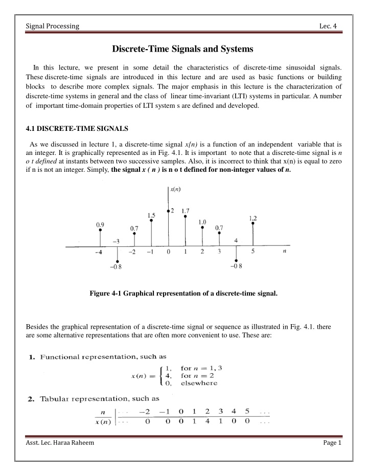
Signal Processing Lec. 4 Discrete-Time Signals and Systems In this lecture, we present in some detail the characteristics of discrete-time sinusoidal signals. These discrete-time signals are introduced in this lecture and are used as basic functions or building blocks to describe more complex signals. The major emphasis in this lecture is the characterization of discrete-time systems in general and the class of linear time-invariant (LTI) systems in particular. A number of important time-domain properties of LTI system s are defined and developed. 4.1 DISCRETE-TIME SIGNALS As we discussed in lecture 1, a discrete-time signal x{n) is a function of an independent variable that is an integer. It is graphically represented as in Fig. 4.1. It is important to note that a discrete-time signal is n o t defined at instants between two successive samples. Also, it is incorrect to think that x(n) is equal to zero if n is not an integer. Simply, the signal x ( n ) is n o t defined for non-integer values of n. Figure 4-1 Graphical representation of a discrete-time signal. Besides the graphical representation of a discrete-time signal or sequence as illustrated in Fig. 4.1. there are some alternative representations that are often more convenient to use. These are: Asst. Lec. Haraa Raheem Page 1

Signal Processing Lec. 4 4.2 Block Diagram Representation of Discrete-Time Systems Asst. Lec. Haraa Raheem Page 2

Signal Processing Lec. 4 Asst. Lec. Haraa Raheem Page 3

Signal Processing Lec. 4 . A Asst. Lec. Haraa Raheem Page 4

Signal Processing Lec. 4 4.3 Response OfADiscrete-Time LTI SystemAnd Convolution Sum A. Impulse Response: The impulse response (or unit sample response) h[n] of a discrete-time LTI system (represented by T) is defined to be the response of the system when the input is ?[n], that is, B. Response to an Arbitrary Input: the input x[n] can be expressed as Since the system is linear, the response y[n] of the system to an arbitrary input x[n] can be expressed as Since the system is time-invariant, we have By substituting: k C. Convolution Sum: Equation (k) defines the convolution of two sequences x[n] and h[n] denoted by j Equation (j) is commonly called the convolution sum. Thus, we have the fundamental result that the output of any discrete-time LTI system is the convolution of the input x[n] with the impulse response h[n] of the system. The Figure below illustrates the definition of the impulse response h[n] and the relationship of Eq. (i). Asst. Lec. Haraa Raheem Page 5

Signal Processing Lec. 4 D. Properties of the Convolution Sum: Convolution is a linear operator and, therefore, has a number of important properties including the commutative, associative, and distributive properties. The definitions and interpretations of these properties are summarized below. 1 . Commutative The commutative property states that the order in which two sequences are convolved is not important. Mathematically, the commutative property is this property states that a system with a unit sample response h(n) and input x(n) behaves in exactly the same way as a system with unit sample response x(n) and an input h(n). This is illustrated in Figure 4.8(a). 2. Associative: The convolution operator satisfies the associative property, which is the associative property states that if two systems with unit sample responses 1(n) and h2(n) are connected in cascade as shown in Figure 4.8 (b), an equivalent system is one that has a unit sample response equal to the convolution of 1(n) and h2(n) : 3. Distributive: The distributive property of the convolution operator states that this property asserts that if two systems with unit sample responses 1(n) and h2(n) are connected in parallel, as shown in Figure 4.8 (c), an equivalent system is one that has a unit sample response equal to the sum of 1(n) and h2(n) Asst. Lec. Haraa Raheem Page 6

Signal Processing Lec. 4 Figure (4.8) The interpretation of convolution properties E. Performing Convolutions There are several different approaches that may be used, and the one that is the easiest will depend upon the form and type of sequences that are to be convolved. 1. Analytical Technique if we want to evaluate y[n] =x[n]* h[n], where x[n] and h[n] are shown in Figure by an analytical technique Asst. Lec. Haraa Raheem Page 7

Signal Processing Lec. 4 2.GraphicalApproach The steps involved in using the graphical approach are as follows: Plot both sequences, x(k) and h(k), as functions of k. Choose one of the sequences, say h(k), and time-reverse it to form the sequence h(-k). Shift the time-reversed sequence by n. [Note: If n > 0, this corresponds to a shift to the right (delay), whereas if n < 0, this corresponds to a shift to the left] Multiply the two sequences x(k) and h(n - k) and sum the product for all values of k. The resulting value will be equal to y(n). This process is repeated for all possible shifts, n. Ex 1: To illustrate the graphical approach to convolution, let evaluate y(n) = x(n)*h(n) where x(n) and h(n) are the sequences shown in Figure 4.9 (a) and (b), respectively. To perform this convolution, we follow the steps listed above : 1.Because x(k) and h(k) are both plotted as a function of k in Figure 4.9 (a) and (b), we next choose one of the sequences to reverse in time. In this example, we time-reverse h(k), which is shown in Figure 4.9 (c). 2. Forming the product, x(k)h(-k), and summing over k, we find that y(0) = 1. Asst. Lec. Haraa Raheem Page 8

Signal Processing Lec. 4 3.Shifting h(k) to the right by one results in the sequence h(l - k ) shown in Figure 4.9(d). Forming the product, x(k)h(l - k), and summing over k, we find that y(1) = 3. 4.Shifting h(l - k) to the right again gives the sequence h(2 - k) shown in Figure 4.9 (e). Forming the product, x(k)h(2 - k), and summing over k, we find that y(2) = 6. 5. Continuing in this manner, we find that y(3) = 5. y(4) = 3, and y(n) = 0 for n > 4. 6. We next take h(-k) and shift it to the left by one as shown in Figure 4.9 (f ). Because the product, x(k)h(- 1 - k), is equal to zero for all k, we find that y(- 1 ) = 0. In fact, y(n) = 0 for all n < 0. Figure 4.9 (g) shows the convolution for all n. Figure 4.9: The graphical approach to convolution. Asst. Lec. Haraa Raheem Page 9

Signal Processing Lec. 4 Auseful fact to remember in performing the convolution of two finite length sequences is that if x(n) is of length L1 and h(n) is of length L2, y(n) = x(n) * h(n) will be of length: L = L1 + L2 1 Ex 2: Evaluate y[n] = x[n] * h[n], where x[n] and h[n] are shown in Fig. by a graphical method. Sol: Asst. Lec. Haraa Raheem Page 10

Signal Processing Lec. 4 Example 3: Using the following sequences defined in Figure , evaluate the digital convolution. a. By the graphical method. b. By applying the formula directly. Sol: Asst. Lec. Haraa Raheem Page 11

Signal Processing Lec. 4 b. Applying Equation (i) with zero initial conditions leads to y(n) = x(0)h(n) + x(1)h(n _ 1)+ x(2)h(n _ 2) H.W: Using the sequence definitions Asst. Lec. Haraa Raheem Page 12

Signal Processing Lec. 4 3.Tabular Method example 3 can be solved by table method as shown in figure below h(n) x(n) 4. Matrix by Vector method y(n) h(n N2 N1+N2-1 N1+N2-1 = [ ] [ ] [ ] N2 Ex 4: If x(n) = [ 0.5 0.5 0.5 ], and h(n) = [ 3 2 1] Ex 5: If h(n) = [ 1 -1 2 ], and x(n) = [ 2 1 -1 3 ] Sol: 2 1 0 2 1 0 0 2= 2 1 1 1 2 6 = 1 2 3 0 1 1 3 0 1 3 ] 5 [ 0 [ ] 6] [ Asst. Lec. Haraa Raheem Page 13

Signal Processing Lec. 4 O=O1+O2-1=position of cursor in y(n), where O1=cursor position in h(n) & O2=cursor position in x(n) For previous example, O=2+3-1=4 cursor position in y(n)={2 -1 2 6 -5 6} 5-Z-Transform Method Y(z)=X(z) H(z) 4.4 Difference Equations and Impulse Responses A causal, linear, time-invariant system can be described by a difference equation having the following general form: b Where a , . . . , a and b , b , . . . , b are the coefficients of the difference equation. Equation (b) can further 1 N 0 1 M be written as: f Notice that y(n) is the current output, which depends on the past output samples y(n 1), . . . , y(n N), the current input sample x(n), and the past input samples, x(n 1), . . . , x(n M). Example1: Given a linear system described by the difference equation y(n) = x(n) + 0.5x(n 1), Determine the nonzero system coefficients. Solution: a. By comparing Equation (f), we have, b = 1, and b = 0.5 0 1 Asst. Lec. Haraa Raheem Page 14

Signal Processing Lec. 4 4.5 System Representation Using Its Impulse Response A linear time-invariant system can be completely described by its unit-impulse response, which is defined as the system response due to the impulse input (n) with zero initial conditions, depicted in Figure below Here x(n) = (n) and y(n) = h(n). Example 2: Given the linear time-invariant system y(n) = 0.5x(n) + 0.25x(n 1) with an initial condition x( 1) = 0 a. Determine the unit-impulse response h(n). b. Draw the system block diagram. c. Write the output using the obtained impulse response. Solution: a. h(n) = 0.5 (n) + 0.25 (n 1) , where h(0)= 0.5, h(1) = 0.25 and h(n) = 0 elsewhere. b. c. y(n) = h(0) x(n) + h(1) x( n 1) From this result, it is noted that if the difference equation without the past output terms, y(n 1), . . . , y(n N), that is, the corresponding coefficients a , . . . , a , are zeros, the impulse response h(n) has a finite 1 number of terms. We call this a finite impulse response (FIR) system. In general, we can express the output sequence of a linear time-invariant system from its impulse response and inputs as: y(n) = . . .. + h( 1) x(n+ 1) + h(0) x(n) + h(1) x(n 1) + h(2) x(n 2) + . . . .. Equation (j) is called the digital convolution sum. N (j) Example 3: For each of the following linear systems, find the unit-impulse response, and draw the block diagram. a. y(n) = 5x(n -10) b. y(n) = x(n) + 0.5x(n - 1) Sol: a. h(n) = 5 (n 10) , where h(10) = 5 and h(n) = 0 elsewhere. h(n)=5?(? 10) Asst. Lec. Haraa Raheem Page 15

Signal Processing Lec. 4 H.W : Compute the convolution y(n) = x(n) * h(n) of the following signals Asst. Lec. Haraa Raheem Page 16