Disruption in Automotive Industry - Strategic Analysis and Impact
In-depth analysis of disruptive technology and climate change in the automotive sector, focusing on key issues, alternatives, and recommendations. Explore the impact of direct sales models and the evolving landscape of the industry.

Download Presentation

Please find below an Image/Link to download the presentation.
The content on the website is provided AS IS for your information and personal use only. It may not be sold, licensed, or shared on other websites without obtaining consent from the author.If you encounter any issues during the download, it is possible that the publisher has removed the file from their server.
You are allowed to download the files provided on this website for personal or commercial use, subject to the condition that they are used lawfully. All files are the property of their respective owners.
The content on the website is provided AS IS for your information and personal use only. It may not be sold, licensed, or shared on other websites without obtaining consent from the author.
E N D
Presentation Transcript
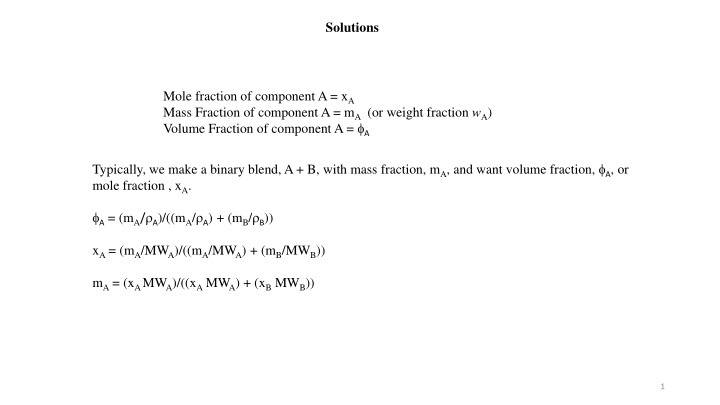
Solutions Mole fraction of component A = xA Mass Fraction of component A = mA (or weight fraction wA) Volume Fraction of component A = A Typically, we make a binary blend, A + B, with mass fraction, mA, and want volume fraction, A, or mole fraction , xA. A= (mA/ A)/((mA/ A) + (mB/ B)) xA = (mA/MWA)/((mA/MWA) + (mB/MWB)) mA = (xA MWA)/((xA MWA) + (xB MWB)) 1
-S U V H A -p G T Solutions We need the free energy of mixing to determine equilibrium G = H TS A = U ST; U = H PV We can measure H and P and V and T but not S Need the Entropy S Three ways to get entropy and free energy of mixing A) Isothermal free energy expression, pressure expression B) Isothermal volume expansion approach, volume expression C) From statistical thermodynamics 2
-S U V H A -p G T A. Pressure Expression: Mix two ideal gasses, A and B p = pA + pB pA is the partial pressure pA = xAp (Raoult s Ideal Mixing Law) For single component molar G = 0 is at p0,A= 1 bar At pressure pA for a pure component isothermal ideal gas = = 0,A + RT ln(p/p0,A) = = 0,A + RT ln(p) dG=-SdT+Vdp Isothermal and Ideal Gas dG = RTdp/p G = RT ln(p/p0) For a mixture of A and B with a total pressure ptot = p0,A = 1 bar and pA = xA ptot For component A in a binary mixture ( (xA) ) = = 0.A + RT ln (xA ptot/p0,A) = = 0.A + RT ln (xA) Isothermal ideal gas (no enthalpy) Notice that xA must be less than or equal to 1, so ln xA must be negative or 0 So, the chemical potential must drop in the solution for a solution to exist. Ideal gasses only have entropy so entropy drives mixing in this case. This can be written, xA = exp(( (xA) 0.A)/RT) Which indicates that xA is the Boltzmann probability of finding A 3
Mix two real gasses, A and B Gas Solution A* = 0.Aif p = 1 4
-S U V H A -p G T Solutions G = H TS A = U ST U = H PV Need the Entropy S Three ways to get entropy and free energy of mixing A) Isothermal free energy expression, pressure expression B) Isothermal volume expansion approach, volume expression C) From statistical thermodynamics 5
B. Volume Expression: Ideal Gas Mixing -S U V H A -p G T For isothermal U = CV dT = 0 = dQ + dW dQ = -dW = pdV For ideal gas dQ = -dW = nRTln(Vf/Vi) dU=-pdV+TdS Isothermal and Ideal Gas dG = RTdp/p dQ = T S S = nR ln(Vf/Vi) Consider a process of expansion of a gas from VA to Vtot The change in entropy is SA = nARln(Vtot/VA) = - nARln(VA/Vtot) Consider an isochoric mixing process of ideal gasses A and B. A is originally in VA and B in VB Vtot is VA + VB The change in entropy for mixing of A and B is Smixing A and B = - nARln(VA/Vtot) - nBRln(VB/Vtot) = - nR(xAlnxA + xBlnxB) For an isothermal, isochoric mixture of ideal gasses (also isobaric since P ~ T/V) For ideal gasses Hmixing = 0 since there is no interaction Gmixing = Hmixing - T Smixing = - T Smixing = nRT(lnxA + lnxB) So, the molar Gibbs Free energy for mixing is Gmixing = RT(xAlnxA + xBlnxB) 6
-S U V H A -p G T Solutions G = H TS A = U ST U = H PV Need the Entropy S Three ways to get entropy and free energy of mixing A) Isothermal free energy expression, pressure expression B) Isothermal volume expansion approach, volume expression C) From statistical thermodynamics 7
C. Statistical Thermodynamics Boltzmann s Law: S = kBln Is the number of states For mixing of nA and nB with n total molecules = n!/(nA! nB!) Sterling s approximation for large n, ln(n!) ~ n ln(n) n We assume that n is large then ln = n ln(n) - (nA ln(nA) + nB ln(nB)) = (nA + nB) ln(n) - (nA ln(nA) + nB ln(nB)) ln = -(nA ln(nA/n) + nB ln(nB/n)) S = -kB (nA ln(nA/n) + nB ln(nB/n)) = -nkB (xA ln(xA) + xB ln(xB)) Gmixing = Hmixing - T Smixing = - T Smixing = nRT(xA lnxA + xB lnxB) 8
Some Types of Entropy Thermodynamic entropy measured experimentally, Q/T Configurational also called Combinatorial Conformational Translational and Rotational Entropy (Brownian motion) Vibrational entropy Conformational entropy computed in internal or Cartesian coordinates (which can even be different from each other) Conformational entropy computed on a lattice Entropy associated with organization on mixing (Hyrophobic effect and many other unexpected features on mixing) 9
-S U V H A -p G T An Ideal Solution means: The change on mixing: S = -nkB (xA ln(xA) + xB ln(xB)) Since (ln x) is always negative or 0, S is always positive for ideal solutions G = -T S Since (ln x) is always negative or 0, G is always negative (or 0) and ideal solutions always mix H is 0, there is no interaction in ideal mixtures, there is no excluded volume, particles are ghosts to each other V = (d G/dp)T = 0, there is no loss or gain of volume compared to the summed volume 10
-S U V H A -p G T Boltzmann Probability of a Thermally Reversible Event = exp(- G/kT) G is the change in free energy for the event G = H T S (Const. T & P, e.g. an experimental measurement) A = U T S (Const. T & V, e.g. a simulation on a grid) Consider an ideal gas with no enthalpic interactions, H = 0 The probability of finding an atom A in a mixture of A and B is the molar concentration xA SA/k = -ln xA from the Boltzmann probability and S/k = - xAln xA - xBln xB by a rule of random mixtures Gideal/kT = xAln xA + xBln xBthis is always negative since ln of a number less than 1 is negative, so mixing always reduces the free energy so it always occurs for an ideal mixture Hildebrandt Real Solution model considers binary interactions. The odds of a binary interaction of A and B is xAxB This interaction has an average enthalpy (or internal energy) H = xAxB AB or x1x2 12 Where the first term is the Hildebrandt binary interaction parameter and the second is the Margules one-parameter interaction term. For polymers 12 is used, the Flory Huggins interaction parameter (with a few modifications). Greal solution/kT = x1ln x1 + x2ln x2 + x1x2 12 = x1ln a1 + x2ln a2 = x1ln 1x1 + x2ln 2x2 H /kT = Gexcess /kT = x1x1 12 = x1ln 1 + x2ln 2 11
Excess free energy per mole GE is the excess free energy value, so nGE The excess chemical potential of component i in phase L or V, iE is given by This is how you can find the activity coefficients from the Margules one-parameter coefficient (or the Hildebrandt or Flory-Huggins interaction parameters) 12
Real Solutions Molar excess functions or departure functions: Difference between real value and ideal value Excess Gmixing = Gmixing - RT(xAlnxA + xAlnxB) Excess Smixing = Smixing + R(xAlnxA + xAlnxB) Excess Hmixing = Hmixing Excess Vmixing = Vmixing 13
Real Solutions xA becomes aA the activity so Gmixing = RT(xAlnaA + xAlnaB) Excess Gmixing = Gmixing - RT(xAlnxA + xBlnxB) = RT(xAln(aA/xA) + xBln(aB/xB) ) = RT(xAln( A) + xBln( B)) Is the activity coefficient Excess Smixing = -R(xAln( A) + xBln( B)) Method to use departure functions for calculations (PREOS.xls) 1) Calculation of properties in the ideal state is simple 2) With an equation of state the departure function can be calculated 3) For any transition first calculate the departure function to the ideal state 4) Then carry out the desired change as an ideal mixture or gas 5) Then use the departure function to return to the real state 14
= RT(xAln(A) + xAln(B)) Gmixing = nRT(xA lnaA + xB lnaB) 15
a = x so da/dx = Get the activity coefficient at infinite dilution by extrapolating the slope for pure component to x = 0 This is used for Henry s Law and a few other places. (Activity coefficient is a/x) 16
We want the infinite dilution activity coefficients to write a function to predict the activity and the activity coefficient. This is one of the parameters for the functions. With the function for activity we can predict the free energy and the miscibility. 17
Solute Solvent or ideal mixture Raoult s Law for solvent or ideal mixtures Vapor pressure = p* xj xj is the solvent molar fraction (high ~1) p* is the vapor pressure of the pure solvent Henry s law for dilute solutions Vapor pressure of solute = ki xi ki is the Henry s Law Constant xi is the solute molar fraction (low ~0) If a solution is ideal, then xA = aA and A = 1 As concentration goes to 1, a solvent is ideal (follows Raoult s law) so (daA/dxA)xA =>1 = 1 = (d AxA/dxA)xA =>1 = A + xA(d A/dxA)xA =>1 But A = 1 at xA = 1, then Raoult s law is followed if (d A/dxA)xA =>1 => 0 (See next slide) A solute follows Henry s Law if (daB/dxB)xB =>0 = Binfinite dilution = (d BxB/dxB)xB =>0 = ( B + xB(d B/dxB))xB =>0 So (xB(d B/dxB))xB =>0 = 0 This isn t that useful 18
Henrys law for dilute solutions Vapor pressure of solute = ki xi Raoult s Law for solvent or ideal mixtures Vapor pressure = p* xj The infinite dilution value comes from the activity plot extrapolation The infinite dilution value comes from the activity plot extrapolation (d B/dxB)xB =>1 => 0 (d A/dxA)xA =>1 => 0 19
You would use Henrian standard state if the solute had limited solubility like PCBs or oil in water and you wanted the infinite dilution of the water component Activity of a component in a solution must be defined relative to a standard state, either Henrian (extrapolated) or Raoultian (measured at x = 1 :: a = 1) 20
Analytic Solution Models Want to calculate the miscibility of components Need to generate a phase diagram Calculation of the vapor pressure Simplest approach could be a polynomial. However, this generally doesn t inherently have any real meaning. The polynomial just reproduces existing data within experimental limits. Extrapolation is dangerous. Asymmetric feature: vapor pressure Symmetric Feature: Phase behavior 21
A Taylor Series Expansion For Example (starting with the infinite dilution value) Excess Gmixing = RT(xAln( A) + xAln( B)) Excess Smixing = -R(xAln( A) + xAln( B)) Interaction coefficients Zeroth order infinite dilution (trivial) First order 1B self-interaction coefficient This is similar to a virial expansion 22
Thallium/Mercury Lower freezing point of Mercury for thermometer and switches 8.5% -60 C versus -40 C Also Rat poison 23
Hildebrand Regular Solution Model The change on mixing: S = -nkB (xA ln(xA) + xB ln(xB)) Ideal Solution Since (ln x) is always negative or 0, S is always positive for ideal solutions G = H -T S Since (ln x) is always negative or 0, G is positive or negative depending on H :: can mix or demix Depending on the sign of H V = (d G/dp)T = 0, there is no loss or gain of volume compared to the summed volume H = n xAxB is the interaction coefficient or regular solution constant Molar Gibbs free energy of mixing Gm = RT(xA ln(xA) + xB ln(xB)) + xAxB = zNA[uAB (uAA+uBB)/2] The equation is symmetric 24
One Crystallographic Phase => + Two Different Crystallographic Phases at Equilibrium 25
N1 N2 Y. Li, M. Stein, B.-J. Jungnickel, Colloid Polym. Sci. 269, 772 (1991); and Mitteilungen aus dem Deutschen Kunststoff- Institut , Nr. 53, April, Darmstadt, 1991 N1 = N2 26
Hildebrand solubility parameter, H = n xAxB is the interaction coefficient or regular solution constant Molar Gibbs free energy of mixing Gm = RT(xA ln(xA) + xB ln(xB)) + xAxB = zNA[uAB (uAA+uBB)/2] Flory-Huggins chi parameter, ~ /kT Hansen solubility parameters 27
Hildebrand Solubility Parameter, Luo Y, Chen X, Wu S, Ca S Luo Z, Shi Y, Molecular Dynamics Simulation Study on Two-Component Solubility Parameters of Carbon Nanotubes and Precisely Tailoring the Thermodynamic Compatibility between Carbon Nanotubes and Polymers, Langmuir 36 9291-9305 (2020). Two materials with similar are miscible Flory-Huggins Equation ~ 1/T Hildebrand and Scratchard London dispersion forces (attractive) 30
Asymmetric equations for asymmetric phase diagram Sub-regular solution model Redlich-Kister Expression 31
Non-ideal entropy of mixing Quasi-regular solution model Greal solution/kT = x1ln x1 + x2ln x2 + x1x2 12 12= 12= A/kT The Margules interaction parameter should have a 1/T dependence, but it often displays a non-combinatorial entropy term 12= /kT + B This can be interpreted that there is some kind of ordering that occurs on mixing Hydrophobic effect is an example. When water and oil are mixed water organizes around oil/water interface reducing the entropy. Entropy depends on number not mass so a large number of water molecules at the interface leads to a large, dominating entropic reduction that causes immiscibility. The enthalpic interaction favors mixing (negative A). A12= 0 at the athermal temperature , T* B = -A/(kT*) 12=( /kT)(1 T/T*) = 12(1 T/T*) T* is a critical temperature 34
From Single Component Systems Slide 34. Landau Theory for Curie transition At the Curie transition (second order transition) Order parameter is 1 at 0 K so and 35
Non-ideal entropy of mixing Quasi-regular solution model This is a non- combinatorial entropy This would occur if there were ordering on mixing, say when you add oil to water. The enthalpy of mixing favors mixing!!! Water organizes at the surface of oil to a great extent; this reduces entropy and makes oil and water demix. Water actually likes oil. This is called the hydrophobic effect and is an important concept for protein folding. 36
Graphical Method to Estimate Chemical Potential Does dG/dxi = dG/dni = i? No dG/dni = dG/dxi dxi/dni dxi/dni = d(ni/(ni+nj))/dni = 1/(ni+nj) ni/(ni+nj)2 37
Solving the Regular Solution Model We know that the excess Gibbs free energy for mixing is given by: GE/RT = xA ln A + xB ln BGeneric expression using activity coefficient And we have defined for the regular solution model that GE/RT = xA xBHildebrand Regular Solution expression If we propose the answer RT ln A = xB2 We find by substitution generic expression that it equals the regular solution expression since xB + xA = 1 (Solving this directly see next slide.) 38
Use of the Gibbs-Duhem Equation to determine the activity of a component Constant p, T Restatement of Gibbs-Duhem for Solutions If you know A you can obtain B by integration 40


 + xAln(B))")