Dynamical Modeling Approaches for Control Analysis and Simulation
Explore different modeling and simulation techniques such as ODEs, PDEs, state machines, and hybrid approaches in control engineering. Understand the importance of models, uncertainty in simulations, and the role of physics-based and input-output models in control systems. Dive into the world of dynamical modeling for practical applications in control engineering.

Download Presentation

Please find below an Image/Link to download the presentation.
The content on the website is provided AS IS for your information and personal use only. It may not be sold, licensed, or shared on other websites without obtaining consent from the author. If you encounter any issues during the download, it is possible that the publisher has removed the file from their server.
You are allowed to download the files provided on this website for personal or commercial use, subject to the condition that they are used lawfully. All files are the property of their respective owners.
The content on the website is provided AS IS for your information and personal use only. It may not be sold, licensed, or shared on other websites without obtaining consent from the author.
E N D
Presentation Transcript
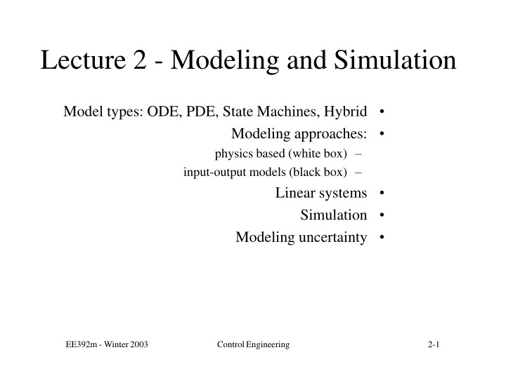
Lecture 2 - Modeling and Simulation Model types: ODE, PDE, State Machines, Hybrid Modeling approaches: physics based (white box) input-output models (black box) Linear systems Simulation Modeling uncertainty EE392m - Winter2003 ControlEngineering 2-1
Goals Review dynamical modeling approaches used for control analysis and simulation Most of the material us assumed to be known Target audience people specializing in controls - practical EE392m - Winter2003 ControlEngineering 2-2
Modeling in Control Engineering Physicalsystem Measurement system Sensors Control ina system perspective Control handles Actuators Control computing Controlanalysis perspective Physical system Control computing Systemmodel Control handle model Measurement model EE392m - Winter2003 ControlEngineering 2-3
Models Model is a mathematical representations of a system Models allow simulating and analyzing the system Models are never exact Modeling depends on your goal A single system may have many models Always understand what is the purpose of the model Large libraries of standard model templates exist A conceptually new model is a big deal Main goals of modeling in control engineering conceptual analysis detailed simulation EE392m - Winter2003 ControlEngineering 2-4
Modeling approaches Controls analysis uses deterministic models. Randomness and uncertainty are usually not dominant. White box models: physics described by ODE and/or PDE Dynamics, Newton mechanics f (x,t) Space flight: add control inputs f (x,u,t) y = g(x,u,t) x = and measured outputs y u x = EE392m - Winter2003 ControlEngineering 2-5
Orbital mechanics example Newton s mechanics fundamental laws dynamics r 3v = m + F (t) pert r v r r = v 1643-1736 r1 r Laplace 2 r3 computationaldynamics (pencil & papercomputations) deterministic model-based x = x = v f (x,t) 1 v2 prediction 1749-1827 2-6 ControlEngineering EE392m - Winter 2003 v3
Orbital mechanics example Space flight mechanics Thrust r v = m +F (t) +u(t) pert 3 r r = v r 1 Control problems: u - ? r 2 state x = r3 observations / measurements control v model 1 v2 (r) x = f (x,u,t) y = g(x,u,t) y = (r) v 3 EE392m - Winter2003 ControlEngineering 2-7
Gene expression model EE392m - Winter2003 ControlEngineering 2-8
Sampled Time Models Time is often sampled because of the digital computer use computations, numerical integration of continuous-time ODE x(t + d) x(t) + d f (x,u,t), digital (sampled time) control system f (x,u,t) t = kd x(t + d) = y = g(x,u,t) Time can be sampled because this is how a system works Example: bank account balance x(t) - balance in the end of day t u(t) - total of deposits and withdrawals that day y(t) - displayed in a daily statement Unit delay operator z-1: z-1 x(t) = x(t-1) x(t +1) = x(t) +u(t) y = x EE392m - Winter2003 ControlEngineering 2-9
Finite state machines TCP/IP StateMachine EE392m - Winter2003 ControlEngineering 2-10
Hybrid systems Combination of continuous-time dynamics and a state machine Thermostat example Tools are not fully established yet x = 70 off on x = 72 x = K (h x)x x = Kx x 70 x 75 x = 75 EE392m - Winter2003 ControlEngineering 2-11
PDE models Include functions of spatial variables electromagnetic fields mass and heattransfer fluid dynamics structural deformations Example: sideways heat equation T = t T (0) =u; x 2T k x2 Tinside=u Toutside=0 T (1) =0 y = T y x heatflux x=1 EE392m - Winter2003 ControlEngineering 2-12
Black-box models Black-box models - describe P as an operator P u y input data output data x internal state AA, ME, Physics - state space, ODE and PDE EE - black-box, ChE - use anything CS - state machines, probablistic models, neural networks EE392m - Winter2003 ControlEngineering 2-13
Linear Systems Impulse response FIR model IIR model State space model Frequency domain Transfer functions Sampled vs. continuous time Linearization EE392m - Winter2003 ControlEngineering 2-14
Linear System (black-box) Linearity u ( ) P y ( ) 1 u ( ) P y( ) 2 1 2 au ( ) + bu ( ) P ay ( ) + by( ) 1 2 2 1 Linear Time-Invariant systems - LTI u( T) P y( T) y u P t t EE392m - Winter2003 ControlEngineering 2-15
Impulse response Response to an input impulse u y ( ) P h( ) t t Sampled time: t = 1, 2, ... Control history = linear combination of the impulses system response = linear combination of the impulse responses u(t) = (t k)u(k) k=0 y(t) = h(t k)u(k) =(h*u)(t) k=0 EE392m - Winter2003 ControlEngineering 2-16
Linear PDE System Example Heat transfer equation, boundary temperature input u heat flux output y Pulse response and step response -2 x 10 PULS E RESPONSE 2T k x2 u = T(0) T t = T (1) =0 Ty = x 6 TEMPERATURE x=1 HEAT FLUX 4 2 1 0.8 0 0 20 60 40 80 100 0.6 TIME S TEP RESPONSE 0.4 1 0.2 0.8 HEAT FLUX 1 0 0 0.6 0.8 0.6 0.2 0.4 0.4 0.4 0.6 0.2 0.8 0.2 0 1 TIME COORDINATE 0 100 80 20 0 40 60 ControlEngineering EE392m - Winter2003 2-17 TIME
FIR model y(t) = hFIR(t k)u(k) =(hFIR*u)(t) N k=0 FIR = Finite Impulse Response Cut off the trailing part of the pulse response to obtain FIR FIR filter state x. Shift register u(t) y(t) h0 z-1 x(t +1) = f (x, u) y = g(x,u) x1=u(t-1) h1 z-1 x2=u(t-2) h2 z-1 x3=u(t-3) h3 EE392m - Winter2003 ControlEngineering 2-18
IIR model nb na y(t) = aky(t k)+ bku(t k) k=0 IIR model: k=1 y(t-1), , y(t-na ), u(t-1), , u(t-nb) Filter states: y(t) u(t) b0 z-1 z-1 y(t-1) u(t-1) -a1 b1 z-1 z-1 y(t-2) u(t-2) -a2 b2 z-1 z-1 y(t-3) u(t-3) -a3 b3 EE392m - Winter2003 ControlEngineering 2-19
IIR model Matlab implementation of an IIR model: filter Transfer function realization: unit delay operator z-1 y(t) = H (z)u(t) + b z 1 + ...+ b b z N + b z N 1 + ... +b z N B(z) 1 b = = H(z) = 1 0 N 0 N 1 + ...+ a 1 +a z + a z N 1 + ... +a zN z N A(z) 1 1 N N z N )u(t) z N )y(t)=(b 0 1 N (1 + a z 1 + ... + a + b z 1 + ...+ b N 1 A(z) B(z) A(z) =1 (or zN) FIR model is a special case of an IIR with EE392m - Winter2003 ControlEngineering 2-20
IIR approximation example Low order IIR approximation of impulse response: (prony in Matlab Signal ProcessingToolbox) Fewer parameters than a FIR model Example: sideways heat transfer pulse response h(t) approximation with IIR filter a = [a1 a2 ], b=[b0 b1 b2 b3 b4] IMP ULSE RESPONSE + b z 4 + b z 1+ b z 2+ b z 3 0 2 3 b 0.06 H(z) = 4 1 11 +a z + a z 2 2 1 0.04 0.02 0 0 20 40 60 80 100 TIME EE392m - Winter2003 ControlEngineering 2-21
Linear state space model x(t +1) = f (x,u, t) y = g(x,u,t) Generic state space model: x(t +1) y(t) = Ax(t) + Bu(t) = Cx(t) + Du(t) LTI state space model another form of IIR model physics-based linear system model y = (Iz A) 1B + D u H(z) = (Iz A) 1B + D Transfer function of an LTI model defines an IIR representation Matlab commands for model conversion: help ltimodels EE392m - Winter2003 ControlEngineering 2-22
Frequency domain description y = H(z)u Sinusoids are eigenfunctions of an LTI system: LTI Plant z 1ei t = ei (t 1)= e i ei t Frequency domain analysis u = u~( )ei td y = H(ei )u~( )ei td ~ y( ) Packet ei t u~( ) Packet ei t ~y( ) y H(ei ) of u of sinusoids sinusoids EE392m - Winter2003 ControlEngineering 2-23


")


