Econometric Analysis of Panel Data for Time Series Applications

This material presents an in-depth examination of econometric analysis applied to panel data for time series applications. Topics covered include cross-country growth convergence, fixed effects models, heterogeneous dynamic models, and more.

• Econometrics
• Panel Data
• Time Series
• Fixed Effects
• Heterogeneous Models

wkisi Follow

Uploaded on Mar 13, 2025 | 0 Views

Download Presentation

Please find below an Image/Link to download the presentation.

The content on the website is provided AS IS for your information and personal use only. It may not be sold, licensed, or shared on other websites without obtaining consent from the author.If you encounter any issues during the download, it is possible that the publisher has removed the file from their server.

You are allowed to download the files provided on this website for personal or commercial use, subject to the condition that they are used lawfully. All files are the property of their respective owners.

The content on the website is provided AS IS for your information and personal use only. It may not be sold, licensed, or shared on other websites without obtaining consent from the author.

Presentation Transcript

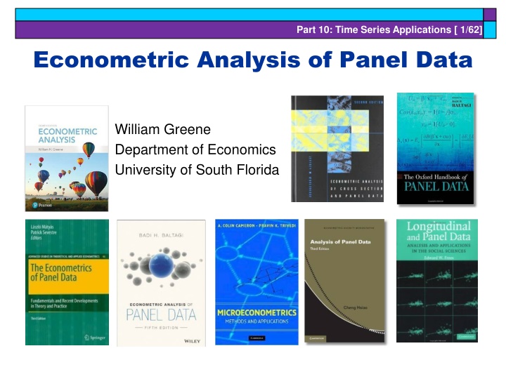
1. Part 10: Time Series Applications [ 1/62] Econometric Analysis of Panel Data William Greene Department of Economics University of South Florida

2. Part 10: Time Series Applications [ 2/62] Time Series Applications Panel Data Time Series Models Univariate Time Series Autocorrelation in Regression Vector Autoregression ARCH and GARCH Models Macroeconomic Data Nonstationarity and Integrated Series Unit Roots Cointegration

3. Part 10: Time Series Applications [ 3/62] Cross Country Growth Convergence Solow - Swan Growth Model 1 = = = Y A K K (A L ) index of technology capital stock = I s Y Investment labor (1 = + i,t i,t i,t i,t i,t + (1- )K Savings = i,t i,t-1 i,t-1 = = i,t 1 I L Equilibrium Model for Steady logY t (1- )g , g=technological growth rate "convergence" parameter; 1- = rate of convergence to steady state Cross country comparisons of convergence rat i,t 1 i = n)L i,t 1 i,t i State Income = + + + logY i,t 1 i,t i i i i,t = = i i i i i i es are the focus of study.

4. Part 10: Time Series Applications [ 4/62] A Heterogeneous Dynamic Model = + + + logY logY x i,t 1 i,t i i i it i,t = Long run effect of interest is i i 1 i Average (over countries) effect: or 1 (1) "Fixed Effects:" Separate regressions, then average results. (2) Country means (o ver time) - can be manipulated to produce consistent estimators of desired parameters (3) Time series of means across countries (does not work at all) (4) Pooled - no way to obtain consistent est (5) Mixed Fixed (Weinhold - Hsiao): Build separate into the equation with "fixed effects," treat imates. i = + u as random. i i

5. Part 10: Time Series Applications [ 5/62] Fixed Effects Approach = + + + logY logY x i,t 1 i,t i i i it i,t = , = i i 1 1 i , (1) Separate regressions; , i i i 1 N 1 N = N i 1 = N i 1 = = (2) Average estimates = or i i 1 i N i 1 = (1/N) (1/N) Function of averages: =1 In each case, each term i has variance O(1/T) i N i 1 = i i N Each average has variance O(1/N) (1/N)O(1/T) i i=1 Expect consistency of estimates of long run effects.

6. Part 10: Time Series Applications [ 6/62] Country Means (Average the T observations for each i) = + i + + logY logY x i,t i i i,t 1 i it i,t = i , = i 1 1 = + i + + logY logY x i i i, 1 i i i Estimates are inconsistent. But, logy logY T logy logY T contains logY i i, 1 T t 1 = , = it i i T t 2 T y y = i,t 1 i,T i,0 = = = logY log Y (y) / T i, 1 i i T i i i = + = 1 + + = + i + + logY logY x (logY (y) / T) x i i i i, 1 i i i i i i T i i i i + + x (y) / T i i i i i i T i 1 1 1 i i i

7. Part 10: Time Series Applications [ 7/62] Country Means (cont.) = + i + + logY logY x i i i, 1 i i i T y y (y) T i,T i,0 = + i + + = (logY (y) / T) x 0 T i i T i i i i i i / (1 ) and ), expect i = + + x (y) / T i i i i i i T i 1 1 1 1 i i i i 0 0 0 = i (1 i (1) Let = = / to be random i i i to be random i i (2) Level variable x should be uncorrelated with change (logY (y) / T). i i T i 0 Regression of logY on 1, x should give consistent estimates of and . i i

8. Part 10: Time Series Applications [ 8/62] Time Series of Means (Average across countries) N = logy (1 /N) logy t = i 1 i,t N N N + + = + (1/N) y (1/N) x (1/N) = i 1 = i 1 ) then = i 1 i,t i i,t 1 i i,t N logy = + = logy Use =(1/N) (1/N) so ( = i 1 i i i N N + i (1/N) ( )logy = i 1 = i 1 i i,t 1 1,t i,t 1 N Likewise for (1/N) x = i 1 i i,t x N = + + + + ( i logy Disturbance is correlated with the regressor. There is no way out, and by construction no instrumental variable that could be correlated with the regressor and not the disturbance. This is hopeless. logy (1/N) ( )logy ...) t = i 1 1,t t t i,t 1

9. Part 10: Time Series Applications [ 9/62] Pooling Essentially the same as the time series case. OLS and GLS are inconsistent There could be no instrument that would work (by construction)

10. Part 10: Time Series Applications [ 10/62] A Mixed/Fixed Approach N = + i + + logy d = country specific dummy variable. Treat and as random, is a 'fixed effect.' This model can be fit consistently by OLS and efficiently by GLS. d logy x = i 1 i,t i i,t i,t 1 i i,t i,t i,t i i i

11. Part 10: Time Series Applications [ 11/62] A Mixed Fixed Model Estimator N = + = + i Heteroscedastic : Var[w x Use two step least squares. (1) Linear regression of logy on dummy variables, dummy i,t-1 variables times logy and x . (2) Regress squares of OLS residuals on x and 1 to + + + logy d logy x (w x ) = i 1 i,t i i i,t i,t 1 i,t i i,t i,t w i 2 w 2 i,t 2 + + ]= x i i,t i,t i,t i,t 2 i,t 2 w 2 estimate (3) Return to (1) but now use weighted least squares. and .

12. Part 10: Time Series Applications [ 12/62]

13. Part 10: Time Series Applications [ 13/62] Nair-Reichert and Weinhold on Growth Weinhold (1996) and Nair Reichert and Weinhold (2001) analyzed growth and development in a panel of 24 developing countries observed for 25 years, 1971 1995. The model they employed was a variant of the mixed-fixed model proposed by Hsiao (1986, 2003). In their specification, GGDPi,t= i + i dit GGDPi,t-1 + 1i GGDIi,t-1 + 2i GFDIi,t-1 + 3i GEXPi,t-1 + 4 INFLi,t-1 + i,t = Growth rate of gross domestic product, = Growth rate of gross domestic investment, = Growth rate of foreign direct investment (inflows), = Growth rate of exports of goods and services, = Inflation rate. GGDP GGDI GFDI GEXP INFL The constant terms and coefficients on the lagged dependent variable are country specific. The remaining coefficients are treated as random, normally distributed, with means kand unrestricted variances. They are modeled as uncorrelated. The model was estimated using a modification of the Hildreth Houck Swamy method

14. Part 10: Time Series Applications [ 14/62] = + w ki k k ki ~ [0,1] w N ki 0.757 5.67 6.45 22.18

15. Part 10: Time Series Applications [ 15/62] Heterogeneous Dynamic Models = + + + logY logY x i,t 1 i,t i i i it i,t = long run effect of interest is i i 1 i See: Pesaran,H.,Smith,R.,Im,K.,"Estimating Long-Run Relationships From Dynamic Heterogeneous Panels," Journal of Econometrics, (Repeated with further study in Matyas and Sevestre, The Econometrics of Panel Data. Smith, J., notes, Applied Econometrics, Dynamic Panel Data Models, University of Warwick. http://www2.warwick.ac.uk/fac/soc/economics/staff/faculty/jennifersmith/panel/ Weinhold, D., "A Dynamic "Fixed Effects" Model for Heterogeneous Panel Data," London School of Economics, 1999. 1995.

16. Part 10: Time Series Applications [ 16/62] TIME SERIES DATA TIME SERIES DATA

17. Part 10: Time Series Applications [ 17/62] Modeling an Economic Time Series Observed y0, y1, , yt, What is the sample Random sampling? The observation window

18. Part 10: Time Series Applications [ 18/62] Estimators Functions of sums of observations Law of large numbers? Nonindependent observations What does increasing sample size mean? Asymptotic properties? (There are no finite sample properties.)

19. Part 10: Time Series Applications [ 19/62] Interpreting a Time Series Time domain: A process y(t) = ax(t) + by(t-1) + Regression like approach/interpretation Frequency domain: A sum of terms y(t) = Contribution of different frequencies to the observed series. ( High frequency data and financial econometrics frequency is used slightly differently here.) ( ) + ( ) Cos t t j j j

20. Part 10: Time Series Applications [ 20/62] For example,

21. Part 10: Time Series Applications [ 21/62] Decomposed

22. Part 10: Time Series Applications [ 22/62] Studying the Frequency Domain Cannot identify the number of terms Cannot identify frequencies from the time series Deconstructing the variance, autocovariances and autocorrelations Contributions at different frequencies Apparent large weights at different frequencies Using Fourier transforms of the data Does this provide new information about the series?

23. Part 10: Time Series Applications [ 23/62] Stationary Time Series zt = b1yt-1 + b2yt-2+ + bPyt-P + et Autocovariance: k = Cov[yt,yt-k] Autocorrelation: k = k / 0 Stationary series: k depends only on k, not on t Weak stationarity: E[yt] is not a function of t, E[yt * yt-s] is not a function of t or s, only of |t-s| Strong stationarity: The joint distribution of [yt,yt-1, ,yt-s] for any window of length s periods, is not a function of t or s. A condition for weak stationarity: The smallest root of the characteristic polynomial: 1 - b1z1 - b2z2 - - bPzP = 0, is greater than one. The unit circle Complex roots Example: yt = yt-1 + ee, 1 - z = 0 has root z = 1/ , | z | > 1 => | | < 1.

24. Part 10: Time Series Applications [ 24/62] The characteristic polynomial is 1 - 1.220175z - (-0.262198)z2 = 0

25. Part 10: Time Series Applications [ 25/62] Side Issue How does y(t) = 1.220175 y(t-1) - 0.262198 y(t-2) + a behave? y(t) = 1.220175 y(t-1) + a is obviously explosive. 1.220175 How to tell: = 1 Smallest (possibly complex) root must be greater than 1.0. 0.262198 0 A

26. Part 10: Time Series Applications [ 26/62] Stationary (et) vs. Nonstationary (yt) Series

27. Part 10: Time Series Applications [ 27/62] The Lag Operator Lc = c when c is a constant Lxt = xt-1 L2 xt = xt-2 LPxt + LQxt = xt-P + xt-Q Polynomials in L: yt = B(L)yt + et e.g., B(L) = (1.22L 0.262L2) A(L) yt = et Invertibility: yt = [A(L)]-1 et

28. Part 10: Time Series Applications [ 28/62] Inverting a Stationary Series yt= yt-1 + et (1- L)yt = et yt = [1- L]-1 et = et + et-1 + 2et-2+ 1 L= + ) ( + + + 2 3 1 ( ) ( ) ... L L L 1 Stationary series can be inverted Autoregressive vs. moving average form of series

29. Part 10: Time Series Applications [ 29/62] VECTOR VECTOR AUTOREGRESSION AUTOREGRESSION

30. Part 10: Time Series Applications [ 30/62] Vector Autoregression The vector autoregression (VAR) model is one of the most successful, flexible, and easy to use models for the analysis of multivariate time series. It is a natural extension of the univariate autoregressive model to dynamic multivariate time series. The VAR model has proven to be especially useful for describing the dynamic behavior of economic and financial time series and for forecasting. It often provides superior forecasts to those from univariate time series models and elaborate theory-based simultaneous equations models. Forecasts from VAR models are quite flexible because they can be made conditional on the potential future paths of specified variables in the model. In addition to data description and forecasting, the VAR model is also used for structural inference and policy analysis. In structural analysis, certain assumptions about the causal structure of the data under investigation are imposed, and the resulting causal impacts of unexpected shocks or innovations to specified variables on the variables in the model are summarized. These causal impacts are usually summarized with impulse response functions and forecast error variance decompositions. Eric Zivot: http://faculty.washington.edu/ezivot/econ584/notes/varModels.pdf

31. Part 10: Time Series Applications [ 31/62] VAR = = = + + + + + + + + + + + + ( ) ( ) ( ) ( 1) 1) 1) ( 1) 1) 1) ( 1) 1) 1) ( ) ( ) ( ) x t ( ) t y t y t y t y t y t y t y t y t y t x t x t 1 11 1 12 2 13 3 y t y t 1 1 ( ( ( ( ( ( ( ) ( ) t t 2 21 1 y t 22 2 23 3 2 2 3 31 1 32 2 33 3 3 3 (In Zivot's examples, 1. Exchange rates 2. y(t )=stock returns, interest rates, indexes of industrial production, rate of inflation

32. Part 10: Time Series Applications [ 32/62] VAR Formulation (t) = SUR with identical regressors. Granger Causality: Non ( ) ( ( ) y t y t = ( ) Hypothesis: does not Granger cause : y (t-1) + x(t) + (t) y y zero off diagonal elements in y t y t + ( ( ( ) y t y t + = + + + + + + + + + 1) 1) 1) ( 1) 1) 1 ( 1) 1) ( ) x t x t x t ( ) t y t y t 1 11 1 12 2 13 3 y t 1 1 + ( ( ( ( ) ( ) ( ) ( ) t y t t 2 2 1 1 22 2 23 3 2 2 = 1) y t y t 3 31 1 3 2 2 33 3 3 0 3 = y 2 1 12

33. Part 10: Time Series Applications [ 33/62] Impulse Response (t) = By backward substitution or using the lag operator (text, 943) (t) x(t) x(t-1) x(t-2) +... (ad infinitum) + (t) (t-1) (t-2) + + [ must converge to as P increases. Roots inside unit circle.] Consider a one time shock (impulse) in the system, = Consider the effect of the impulse on y ( ), s=t, t+1,... Ef 2 fect in period t is 0. is not in the y1 equation. affects y2 in period t, which affects y1 in period t+1. Effect is (t-1) + x(t) + (t) y y = + + 2 y 2 + ... P 0 in period t 2 s 1 2 12 2 In period t+2, the effect from 2 periods back is ( ... and so on . ) 12

34. Part 10: Time Series Applications [ 34/62] Zivot s Data

35. Part 10: Time Series Applications [ 35/62] Impulse Responses

36. Part 10: Time Series Applications [ 36/62] ARCH AND GARCH ARCH AND GARCH MODELS MODELS

37. Part 10: Time Series Applications [ 37/62] GARCH Models: A Model for Time Series GARCH Models: A Model for Time Series with Latent Heteroscedasticity with Latent Heteroscedasticity Bollerslev/Ghysel, 1974

38. Part 10: Time Series Applications [ 38/62] ARCH Model

39. Part 10: Time Series Applications [ 39/62] GARCH Model

40. Part 10: Time Series Applications [ 40/62] Estimated GARCH Model ---------------------------------------------------------------------- GARCH MODEL Dependent variable Y Log likelihood function -1106.60788 Restricted log likelihood -1311.09637 Chi squared [ 2 d.f.] 408.97699 Significance level .00000 McFadden Pseudo R-squared .1559676 Estimation based on N = 1974, K = 4 GARCH Model, P = 1, Q = 1 Wald statistic for GARCH = 3727.503 --------+------------------------------------------------------------- Variable| Coefficient Standard Error b/St.Er. P[|Z|>z] Mean of X --------+------------------------------------------------------------- |Regression parameters Constant| -.00619 .00873 -.709 .4783 |Unconditional Variance Alpha(0)| .01076*** .00312 3.445 .0006 |Lagged Variance Terms Delta(1)| .80597*** .03015 26.731 .0000 |Lagged Squared Disturbance Terms Alpha(1)| .15313*** .02732 5.605 .0000 |Equilibrium variance, a0/[1-D(1)-A(1)] EquilVar| .26316 .59402 .443 .6577 --------+-------------------------------------------------------------

41. Part 10: Time Series Applications [ 41/62] MACROECONOMIC DATA MACROECONOMIC DATA

42. Part 10: Time Series Applications [ 42/62] Analysis of Macroeconomic Data Integrated series The problem with regressions involving nonstationary series Spurious regressions Unit roots and misleading relationships Solutions to the problem Random walks and first differencing Removing common trends Cointegration: Formal solutions to regression models involving nonstationary data Extending these results to panels Large T and small T cases. Parameter heterogeneity across countries

43. Part 10: Time Series Applications [ 43/62] Nonstationary Data

44. Part 10: Time Series Applications [ 44/62] Integrated Series

45. Part 10: Time Series Applications [ 45/62] Stationary Data

46. Part 10: Time Series Applications [ 46/62] Integrated Processes Integration of order (P) when the P th differenced series is stationary Stationary series are I(0) Trending series are often I(1). Then yt yt-1 = yt is I(0). [Most macroeconomic data series.] Accelerating series might be I(2). Then (yt yt-1)- (yt yt-1) = 2yt is I(0) Historic Hyperinflations Interwar Germany, Hungary 1946, Zimbabwe 2007-2008 Money stock in hyperinflationary economies. Price level in Venezuela in 2016 - 2017

47. Part 10: Time Series Applications [ 47/62] A Unit Root? How to test for = 1? By construction: t t-1 = ( - 1) t-1 + ut Test for = ( - 1) = 0 using regression? Variance goes to 0 faster than 1/T. Need a new table; can t use standard t tables. Dickey Fuller tests This invokes the possibility of unit roots in economic data. (Are there?) Nonstationary series Implications for conventional analysis

48. Part 10: Time Series Applications [ 48/62] Unit Root Tests = + + + + L l 1 l = y Different restrictions on parameters produce the model. The parameter of interest is . Augmented Dickey-Fuller Tests: Unit root test H : < 1 vs. H : KPSS Tests: Null hypothesis is stationarity. Alternative is broadly defined as nonstationary. y t y t 1 t l t 0 t 0 = 1. 0 1

49. Part 10: Time Series Applications [ 49/62] KPSS Test-1

50. Part 10: Time Series Applications [ 50/62] KPSS Test-2

Load More ...