Efficient Algorithm for Computing DFT Coefficients | Digital Signal Processing
Learn about the efficient algorithm for computing Discrete Fourier Transform (DFT) coefficients known as Fast Fourier Transform (FFT) in the context of Digital Signal Processing. Explore graphical operations, decimation-in-frequency method, and block diagrams for 8-point FFT iterations with examples and solutions provided.

Uploaded on | 1 Views
Download Presentation

Please find below an Image/Link to download the presentation.
The content on the website is provided AS IS for your information and personal use only. It may not be sold, licensed, or shared on other websites without obtaining consent from the author. If you encounter any issues during the download, it is possible that the publisher has removed the file from their server.
You are allowed to download the files provided on this website for personal or commercial use, subject to the condition that they are used lawfully. All files are the property of their respective owners.
The content on the website is provided AS IS for your information and personal use only. It may not be sold, licensed, or shared on other websites without obtaining consent from the author.
E N D
Presentation Transcript
CEN352 Digital Signal Processing BY Dr. Anwar M. Mirza / Office No. 2185 Phone: 4697362 anwar.m.mirza@gmail.com or ammirza@ksu.edu.sa Lecture No. 12 to 14 Department of Computer Department of Computer Engineering, College of Computer and Information Sciences, College of Computer and Information Sciences, King Saud University, Riyadh, Kingdom of Saudi Arabia King Saud University, Riyadh, Kingdom of Saudi Arabia October, 2012 October, 2012 Engineering,
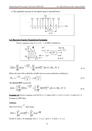
It is a very efficient algorithm for computing the DFT coefficients. Fast Fourier Transform
z=x+y x z=wx z=x y x x y w 1 y Definitions of the graphical operations Method of Decimation-in-Frequency a(0) X(0) x(0) (N/2)- point DFT a(1) X(2) x(1) a(2) X(4) x(2) a3) X(6) x(3) WN0 WN1 WN2 WN3 b(0) X(1) x(4) 1 1 1 1 b(1) (N/2)- point DFT X(3) x(5) b(2) X(5) x(6) b(3) X(7) x(7) The first iteration of the 8-point FFT
Method of Decimation-in-Frequency X(0) x(0) (N/4)- point DFT X(2) x(1) X(4) x(2) (N/4)- point DFT 1 1 WN0 WN2 X(6) x(3) X(1) x(4) (N/4)- point DFT 1 1 1 1 WN0 WN1 WN2 X(3) x(5) X(5) x(6) (N/4)- point DFT 1 1 WN0 X(7) x(7) WN3 WN2 The second iteration of the 8-point FFT
Method of Decimation-in-Frequency x(0) X(0) x(1) X(2) 1 WN0 x(2) X(4) 1 1 x(3) X(6) 1 WN0 x(4) X(1) 1 1 1 1 WN0 WN1 WN2 x(5) X(3) 1 WN0 x(6) X(5) 1 1 WN0 x(7) X(7) 1 WN3 WN2 WN0 Block diagram for the 8-point FFT (total twelve multiplications)
Example 4.12 Solution Bit Reversal Bit Index 4 10 10 = X(0) 00 00 x(0)=1 6 -2 -2 = X(2) 10 01 x(1)=2 W40 = 1 -2+2j -2 -2 -2+2j = X(1) 01 10 x(2)=3 W40 = 1 -2-2j -2 2j -2-2j = X(3) 11 11 x(3)=4 W41 = -j W40 = 1 First Iteration Second Iteration
Example 4.13 Solution Bit Reversal Bit Index 8 10 4 = x(0) 00 00 X(0)=10 -4 -2 12 = x(2) 10 01 X(1)=-2+j2 -2+2j 12 12 8 = x(1) 01 10 X(2)=-2 -2-2j j4 -4 16 = x(3) 11 11 X(3)=-2-j2 First Iteration Second Iteration
Method of Decimation-in-Time The first iteration of the 8-point FFT using Decimation-in-Time
Method of Decimation-in-Time The second iteration of the 8-point FFT using Decimation-in-Time
Method of Decimation-in-Time The 8-point FFT using Decimation-in-Time (12 complex multiplications)
Method of Decimation-in-Time The 8-point IFFT using Decimation-in-Time
Example 4.12 Solution Bit Reversal Bit Index 8 12 12 = X(0) 00 00 x(0)=6 4 4 4 = X(2) 10 01 x(1)=4 W40 = 1 4-4j 4 4 4-4j = X(1) 01 10 x(2)=2 W40 = 1 4+4j 4 -4j 4+4j = X(3) 11 11 x(3)=0 W41 = -j W40 = 1 First Iteration Second Iteration
Example 4.12 Solution Bit Reversal Bit Index 4 10 10 = X(0) 00 00 x(0)=1 6 -2 -2 = X(2) 10 01 x(1)=2 W40 = 1 -2+2j -2 -2 -2+2j = X(1) 01 10 x(2)=3 W40 = 1 -2-2j -2 2j -2-2j = X(3) 11 11 x(3)=4 W41 = -j W40 = 1 First Iteration Second Iteration