Efficient Resistance Distance Computation: Landmark-based Approaches

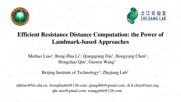
Efficient Resistance Distance Computation: the Power of Landmark-based Approaches Meihao Liao1, Rong-Hua Li1, Qiangqiang Dai1, Hongyang Chen2, Hongchao Qin1, Guoren Wang1 Beijing Institute of Technology1; Zhejiang Lab2 mhliao@bit.edu.cn; lironghuabit@126.com; qiangd66@gmail.com; dr.h.chen@ieee.org; qhc.neu@gmail.com; wanggrbit@126.com

1. Problem Definition Resistance distance Model a graph as an electrical network 2 5 node: junction; edge: resistor 3 1 r(s,t): a unit current flows in through s, flows out through t, the effective resistance between s and t 7 6 4 Resistance distance is a distance metric; Resistance distance is a vertex similarity; Resistance distance captures commute time (expected length of random walk start from s, arrive t and travel back to s) c(s,t) = h(s,t)+h(t,s) = 2m * r(s,t) Our problem: single pair r(s,t) for s,t; single source r(s,u) for s

1. Problem Definition Existing solutions for computing r(s,t) Direct method : r(s,t) = (L )ss+ (L )tt- 2(L )st The inverse of Laplacian matrix does not exist, It s hard to directly compute pseudo-inverse L (O(n^3)!)

1. Problem Definition Existing solutions for computing r(s,t) Direct method : r(s,t) = (L )ss+ (L )tt- 2(L )st The inverse of Laplacian matrix does not exist, It s hard to directly compute pseudo-inverse L (O(n^3)!) Random walk sampling: r(s,t) = c(s,t) Sample random walks from s, arrive t, and back to s The random walk length is too long, takes too much time (2m*r(s,t) for each pair of nodes)

2. Our Solutions A new formula of r( s,t) r u,v =(Lv 1)uu r s,t =(Lv 1)ss+(Lv 1)tt 2(Lv 1)st s,t v Lv: submatrix of L obtained by deleting the v-th row and column of L All pairs of resistance distances can be represented by the inverse of Lv If s,t v, r(s,t) maintains as an invariant, no matter how we choose v Key insight: Choosing v as a landmark node (easy-to-hit) will simplify calculation!

2. Our Solutions Theoretical interpretations of r( s,t) r u,v =(Lv 1)uu r s,t =(Lv 1)ss+(Lv 1)tt 2(Lv 1)st s,t v v-absorbed random walk interpretation v-absorbed random walk: random walk stops when it hits v v(s,u): the number of passes to a node u in a v-absorbed random walk from s r(s,t) = v(s,s) / ds+ v(t,t) / dt- 2 v(s,t) / dt This leads to a simple Monte Carlo algorithm!

2. Our Solutions Theoretical interpretations of r( s,t) r u,v =(Lv 1)uu r s,t =(Lv 1)ss+(Lv 1)tt 2(Lv 1)st s,t v v-absorbed random walk interpretation r(s,t) = v(s,s) / ds+ v(t,t) / dt- 2 v(s,t) / dt This leads to a simple Monte Carlo algorithm! Run a number of v-absorbed random walks from s and t, take the average number of passes to s and t as an estimation of r(s,t). When v is chosen as an easy-to-hit node, the algorithm will terminate very fast!

2. Our Solutions Theoretical interpretations of r( s,t) r u,v =(Lv 1)uu r s,t =(Lv 1)ss+(Lv 1)tt 2(Lv 1)st s,t v v-absorbed push interpretation Push: locally compute a column of A 1(Gauss Seidel algorithm in numerical linear algebra)

2. Our Solutions v-absorbed random walk v4[v2,v1]=0.5 V1 Theoretical interpretations of r( s,t) v4[v2,v2]=1.25 V2 V3 v-absorbed push interpretation can be regarded as a deterministic version of v-absorbed walk v4[v2,v3]=0.25 start from a source node v2, maintain p and r In each step, select a node, add the residual (r) to reserve (p), push the residuals to all its neighbors. Ignore the residual when v is met. V4

2. Our Solutions v-absorbed random walk v4[v2,v1]=0.5 V1 Theoretical interpretations of r( s,t) v4[v2,v2]=1.25 V2 V3 v-absorbed push interpretation can be regarded as a deterministic version of v-absorbed walk v4[v2,v3]=0.25 start from a source node v2, maintain p and r In each step, select a node, add the residual (r) to reserve (p), push the residual to all its neighbors. Ignore the residual when v is met. V4 p - estimation ; r error (used to evaluate error).

2. Our Solutions Theoretical interpretations of r( s,t) r u,v =(Lv 1)uu r s,t =(Lv 1)ss+(Lv 1)tt 2(Lv 1)st s,t v v-absorbed push and v-absorbed random walk can be combined as a bi-directional algorithm Ideas borrowed from personalized PageRank (PPR) First apply v-absorbed push, then simulate v-absorbed random walks based on the residual r. A better algorithm than both v-absorbed walk and v-absorbed push.

2. Our Solutions Theoretical interpretations of r( s,t) spanning tree interpretation matrix forest theorem: det(Lv) = # spanning trees spanning tree centrality: r(e=(s,t))= # spanning trees with edge e / # spanning trees electrical flow is an average of flows on all spanning trees V1 V1 V1 V1 V1 s s s s V3 V3 V3 V2 V2 V2 V3 An example graph G V2 V2 V3 V4 V4 V4 V4 t t t V4 t V1 V1 V1 V1 V1 1/8 3/8 s s s s V3 V2 electrical flow on G V3 V3 V2 V2 V3 V2 s 2/8 V2 V3 1/8 5/8 V4 V4 V4 t V4 t t t V4 t

2. Our Solutions Theoretical interpretations of r( s,t) Sample a spanning tree Aldous-Broder algorithm: simulate a random walk until all nodes are covered Wilson algorithm: simulate a loop-erased walk with root v a local version of Wilson algorithm: simulate a v-absorbed walk from s and t Run a v-absorbed random walk from s, run a v- absorbed walk from t, stops either when hitting v or hitting the loop-erased trajectory of walk from s. Once v-absorbed walks are sampled from s and t, the unique path from s to t in the sampled spanning tree is determined, the eletrical flow is the average of such s-t paths.

2. Our Solutions Single source algorithms for r( s,u) Former algorithms well support single pair query A single source algorithm need to invoke single pair algorithms for n times, which is unnecessary. An existing algorithm: spanning tree sampling. We prove that: The expected number of passes to a node u in a loop-erased walk with root v is (Lv 1)uu. Single source resistance distance from s can be approximated by simulating one single loop-erased walk with root s.

2. Our Solutions Single source algorithms for r( s,u) Index based algorithm r u,v =(Lv 1)uu According to the formula r s,t =(Lv 1)ss+(Lv 1)tt 2(Lv 1)st s,t v Single source resistance distance from s can be solved by building an index of single source resistance distance from landmark node v. v-absorbed walk v-absorbed push With an O(n) index, we can answer a single source resistance distance query in time of answering a single pair query.

3. Experimental Results Single pair resistance distance query Query time Estimation error The bidirectional algorithm that combines v-absorbed push and v- absorbed walk is the best algorithm in terms of query time and error; push is very fast with reasonable error.

3. Experimental Results Single source resistance distance query Estimation error Query time Loop-erased walk sampling is better than spanning tree sampling for the landmark node v; index-based methods are extremely fast.

3. Experimental Results Verify landmark node v single pair single source single source single pair Query time Estimation error We also verify the landmark node v. The results show that the highest degree node in real-life social graphs is a good choice.

Take Home Message Resistance distance can be interpreted as a matrix inverse which is similar to personalized PageRank (PPR), techniques in PPR can be borrowed for solving problems of resistance distance! There are many interesting theoretical interpretations and algorithms for resistance distances!

THANKS