Efficient SQL Query Processing and Database Performance Tuning
Learn how to efficiently implement SQL queries in a relational database system and optimize database performance for better results. Gain essential knowledge for DBA roles at top tech companies like Oracle, Microsoft, IBM, and Google. Explore logical/physical operators, query processing, and query execution plans, along with examples and valuable insights.

Uploaded on | 1 Views
Download Presentation

Please find below an Image/Link to download the presentation.
The content on the website is provided AS IS for your information and personal use only. It may not be sold, licensed, or shared on other websites without obtaining consent from the author. If you encounter any issues during the download, it is possible that the publisher has removed the file from their server.
You are allowed to download the files provided on this website for personal or commercial use, subject to the condition that they are used lawfully. All files are the property of their respective owners.
The content on the website is provided AS IS for your information and personal use only. It may not be sold, licensed, or shared on other websites without obtaining consent from the author.
E N D
Presentation Transcript
COP5725 Advanced Database Systems Query Processing Tallahassee, Florida Tallahassee, Florida
Why Do We Learn This? How to implement (efficiently) SQL queries in a relational database system? As a DBA, how to tune your database system in order to have better performance? Must-know knowledge if you want to get a job in Oracle, Microsoft, IBM, Google, 1
Outline Logical/physical operators Cost parameters and sorting One-pass algorithms Nested-loop joins Two-pass algorithms 2
Query Processing Query or update Query compiler User/Application Query execution plan Execution engine Record, index requests Index/record mgr. Page commands Buffer manager Read/write pages Storage manager storage 3
Logical vs. Physical Operators Logical operators what they do e.g., union, selection, projection, join, grouping, Physical operators how they do it e.g., nested loop join, sort-merge join, hash join, index join 4
Query Execution Plans SELECT S.sname FROM Purchase P, Person Q WHERE P.buyer=Q.name AND Q.city= tallahassee AND Q.phone > 5430000 buyer City= tallahassee phone> 5430000 Query Plan: logical tree implementation choice at every node scheduling of operations Buyer=name (Simple Nested Loops) Person (Index scan) Purchase (Table scan) Some operators are from relational algebra, and others (e.g., sort, scan, group) are not 5
How do We Combine Operators? The iterator model: Each operator is implemented by three functions: Open: sets up the data structures and performs initializations Next: returns the next tuple of the result, or NotFound if there are no more tuples to return Close: ends the operations and cleans up the data structures Enables pipelining! 6
The Iterator Model Query execution always begins with the root iterator Parent.Open() invokes Child.Open() and sometimes Child.Next() Parent.Next() invokes Child.Next() or nothing Parent.Close() invokes Child.Close() 8
Query Execution: Materialization vs. Pipelining Materialization - result of each operator is stored on disk until it is needed by another operator high disk I/O one operation at time Pipelining - result of each operator is created in the main memory and passed directly to operator that uses it save disk I/O operations are performed simultaneously fails when the size of results and intermediate data structures exceed the limits of the main memory 9
Cost Parameters Cost parameters M = number of blocks that fit in main memory B(R) = number of blocks holding R T(R) = number of tuples in R V(R,a) = number of distinct values of the attribute a Estimating the cost: Important in optimization (next lecture) Compute I/O cost only (memory disk) accesses to disks are much slower than accesses to RAM! We compute the cost to read the tables We don t compute the cost to write the result (because pipelining) 10
Classification of Algorithms One-Pass algorithms read the data from disk only once. Work when at least one of the relations fits in the main memory Exception: projection and selection Two-Pass algorithms read the data from disc twice. Work for the data which does not fit in the main memory, but not for the largest imaginable data Sorting-based Hash-based Multi-Pass algorithms read the data three or more times, and are natural, recursive generalizations of the two-pass algorithms. Work without limit on the size of the data 11
Table Scanning If the table is clustered (blocks consists only of records from this table): Table-scan: if we know where the blocks are Cost: B(R) Index scan: if we have index to find the blocks Cost: B(R) If the table is unclustered (its records are placed on blocks with other tables) May need one read for each record Cost: T(R) 12
One-pass Algorithms Selection (R) , projection (R) Both are tuple-at-a-time algorithms Read a block at a time, use one memory buffer and produce the output Cost B(R) if R is clustered T(R) if R is unclustered Assumption: M 1 for the input buffer, regardless of B Unary operator Input buffer Output buffer 13
One-pass Algorithms Duplicate elimination: (R) Need to keep a dictionary in memory in order to maintain one copy of every tuple we have seen: balanced search tree O(n logn) hash table O(n) Memory Requirements 1 buffer to store one block of input tuples M 1 buffers to store one copy of each distinct tuple Cost: B(R) Assumption: B( (R)) <= M 14
One-pass Algorithms Grouping: city, sum(price)(R) Need to keep a dictionary in memory Also store the sum(price) for each city Cost: B(R) Assumption: number of cities fits in memory Binary operations: R S, R U S, R S Assumption: min(B(R), B(S)) <= M One buffer used to read the blocks of the larger relation, while M- 1 buffers needed to house the entire smaller relation and its main memory-data structures Cost: B(R)+B(S) 15
Nested Loop Joins Tuple-based nested loop R S R=outer relation, S=inner relation for each tuple r in R do for each tuple s in S do if r and s joinable joinable then output (r, s) Cost: T(R) T(S), sometimes T(R) B(S) 16
Nested Loop Joins Block-based Nested Loop Join for for each (M for each (M- -1) blocks for each block for for 1) blocks bs bs of S each block br for each tuple s in for each tuple r in if if r and s joinable of S do do do do br of R of R do each tuple s in bs bs do each tuple r in br r and s joinable then br do do then output(r, s) output(r, s) 17
Nested Loop Joins Join Result R & S Blocks of S (k < M-1 pages) . . . . . . . . . Output buffer Input buffer for R 18
Nested Loop Joins Block-based Nested Loop Join Cost: Read S once: cost B(S) Outer loop runs B(S)/(M-1) times, and each time need to read R: costs B(S)B(R)/(M-1) Total cost: B(S) + B(S)B(R)/(M-1) Notice: it is better to iterate over the smaller relation first i.e., S smaller 19
Summary of One-pass Algorithms Operators U, , -, X join M Required 1 B Min(B(R), B(S)) any M 2 Disk I/O B B B(R)+B(S) B(R)B(S)/M 20
Two-pass Algorithm Relations are larger than what the one-pass algorithms can handle Philosophy Pass 1: organize the data properly into a group of sub-relations, and write out to disk again Sorting Indexing Pass 2: reread each sub-relation, do the operation 21
Review: Main-Memory Merge Sort http://www.youtube.com/watch?v=GCae1WNvnZM 22
Sorting 2 Pass Multi-way Merge Sort (2PMMS) Step 1: Read M blocks at a time, sort, write Result: B/M runs of length M on disk (the last run may be shorter) Step 2: Merge M-1 at a time, write to disk (M-1): input buffer 1: output buffer Cost: 3B(R) One read and one write for step 1 One read for merging at step 2 Assumption: B(R) M2 23
Example 24
Example 1G Memory, Block size 64K M = 2^30/ 2^16 = 16K A relation fitting in B blocks can be sorted if B (16K)^2 = 2^28 Each block is 64K Then the largest table affordable is 2^28 * 2^16 = 2^42 bytes = 4 Terabytes! Even on a modest machine, 2PMMS is sufficient to sort all but an incredibly large relation in two passes 25
Two-Pass Algorithms Based on Sorting Duplicate elimination (R) Simple idea: like sorting, but include no duplicates Step 1: sort runs of size M, write Cost: 2B(R) Step 2: merge M-1 runs, but include each tuple only once Cost: B(R) Total cost: 3B(R), Assumption: B(R)<= M2 26
Two-Pass Algorithms Based on Sorting Grouping: city, sum(price)(R) Same as before: sort based on city, then compute the sum(price) for each group As before: compute sum(price) during the merge phase Total cost: 3B(R) Assumption: B(R)<= M2 27
Two-Pass Algorithms Based on Sorting Binary operations: R S, R U S, R S Idea: sort R, sort S, then do the right thing A closer look: Step 1: split R into runs of size M, then split S into runs of size M. Cost: 2B(R) + 2B(S) Step 2: merge all x runs from R; merge all y runs from S; ouput a tuple on a case by cases basis (x + y <= M) Total cost: 3B(R)+3B(S) Assumption: B(R)+B(S)<= M2 28
Two-Pass Algorithms Based on Sorting Join R S Start by sorting both R and S on the join attribute: Cost: 4B(R)+4B(S) (because need to write to disk) Read both relations in sorted order, match tuples Cost: B(R)+B(S) Difficulty: many tuples in R may match many in S If at least one set of tuples fits in M, we are OK Otherwise need nested loop, higher cost Total cost: 5B(R)+5B(S) Assumption: B(R)<= M2, B(S)<= M2 29
Summary of Two-pass Algorithms Based on Sorting Operators M Required Disk I/O 3B ? U, , - 3(B(R)+B(S)) ? ? + ?(?) join 5(B(R)+B(S)) max(? ? ,? ? ) 30
Two Pass Algorithms Based on Hashing Idea: partition a relation R into buckets, on disk Each bucket has size approx. B(R)/M Relation R Partitions OUTPUT 1 1 1 2 INPUT 2 2 hash function h . . . M-1 B(R) M-1 M main memory buffers Disk Disk Does each bucket fit in main memory ? Yes if B(R)/M <= M, i.e. B(R) <= M2 31
Hash Based Algorithms for (R) = = duplicate elimination Step 1. Partition R into buckets Step 2. Apply to each bucket (may read in main memory and apply one-pass algorithm) Cost: 3B(R) Assumption: B(R) <= M2 32
Hash Based Algorithms for (R) = = grouping and aggregation Step 1. Partition R into buckets Choose the hash function depending only on the grouping attributes Step 2. Apply to each bucket (may read in main memory) Cost: 3B(R) Assumption: B(R) <= M2 33
Hash-based Join R S Simple version: main memory hash-based join Scan S, build buckets in main memory Then scan R and join Requirement: min(B(R), B(S)) <= M 34
Partitioned Hash Join R S Step 1: Hash S into M buckets send all buckets to disk Step 2 Hash R into M buckets (the same hash function on join attributes) Send all buckets to disk Step 3 Join every pair of buckets Cost: 3B(R) + 3B(S) Assumption: At least one full bucket of the smaller relation must fit in memory: min(B(R), B(S)) <= M2 35
Partitioned Hash Join Original Relation 1. Partition both Partitions OUTPUT 1 relations using hash 1 2 2 INPUT hash function h function h . . . M-1 R tuples in partition i will only match S tuples in partition i M-1 main memory buffers Disk Disk Partitions of R & S Join Result 2. Read in a partition of Hash table for partition Si ( < M-1 pages) hash fn h2 S, hash it using h2 (<> h!). Scan h2 matching partition of Output buffer Input buffer for Ri R, search for matches main memory buffers Disk Disk 36
Summary of Two-pass Algorithms Based on Hashing Operators M Required Disk I/O 3B ? U, , - 3(B(R)+B(S)) min(? ? ,? ? ) join 3(B(R)+B(S)) min(? ? ,? ? ) 37
Indexed Based Algorithms Zero-pass! In a clustering index all tuples with the same value of the key are clustered on as few blocks as possible a a a a a a a a a a 38
Index Based Selection Selection on equality: a=v(R) Clustered index on a: cost B(R)/V(R,a) Unclustered index on a: cost T(R)/V(R,a) Example: B(R) = 2000, T(R) = 100,000, V(R, a) = 20, compute the cost of a=v(R) Cost of table scan: If R is clustered: B(R) = 2000 I/Os If R is unclustered: T(R) = 100,000 I/Os Cost of index based selection: If index is clustered: B(R)/V(R,a) = 100 If index is unclustered: T(R)/V(R,a) = 5000 Notice: when V(R,a) is small, then unclustered index is useless 39
Index Based Join R S Assume S has an index on the join attribute Iterate over R, for each tuple fetch corresponding tuple(s) from S Assume R is clustered. Cost: If index is clustered: B(R) + T(R)B(S)/V(S,a) If index is unclustered: B(R) + T(R)T(S)/V(S,a) Assume both R and S have a sorted index (B+ tree) on the join attribute Then perform a merge join (called zig-zag join) Cost: B(R) + B(S) 40
Have Fun! Tallahassee, Florida Tallahassee, Florida