Embedded Sensors: Innovative Applications and Coding Solutions
Discover creative uses for embedded sensors in various objects like a radio-controlled race car or hand sanitizer dispenser. Learn how to embed sensors, code solutions, and utilize them effectively. Explore the possibilities of embedding distance, heat, and touch sensors into objects for practical applications.
Download Presentation

Please find below an Image/Link to download the presentation.
The content on the website is provided AS IS for your information and personal use only. It may not be sold, licensed, or shared on other websites without obtaining consent from the author.If you encounter any issues during the download, it is possible that the publisher has removed the file from their server.
You are allowed to download the files provided on this website for personal or commercial use, subject to the condition that they are used lawfully. All files are the property of their respective owners.
The content on the website is provided AS IS for your information and personal use only. It may not be sold, licensed, or shared on other websites without obtaining consent from the author.
E N D
Presentation Transcript
FracMeet III, IMSc, Chennai, 21-24 January, 2013 Scaling forms for Relaxation Times of the Fiber Bundle Model S. S. Manna In collaboration with C. Roy,S. Kundu and S. Pradhan Satyendra Nath Bose National Center for Basics Sciences, Kolkata SINTEF Petroleum Research, Trondheim, Norway
FIBER BUNDLE MODEL What is a fiber bundle? Fiber bundle models study breakdown properties of a bundle composed of a large number of N parallel elastic fibers. Arrangement All fibers of the bundle are rigidly clamped at one end and is externally loaded at the other end. The load is equally distributed among all fibers. Disorder Each fiber i has a breaking threshold bi of its own. If the stress acting through it exceeds bi the fiber breaks. The bi values are drawn from a distribution p(b) whose cumulative distribution is 0 b = P(b) p(b)db
STRESS RELAXATION Suppose is the external load per fiber applied on a complete bundle. Then the fibers having breaking thresholds bi < would break. They release the total amount of stress that were acting through them. The released stress gets distributed among some other fibers. In the Equal Load Sharing (ELS) version the released stress is equally distributed among all intact fibers. This is one time step. If the new stress per fiber is then there will be another set of fibers which will break again and release stress. A cascade of such activities follows for T time steps which stops when the system reaches a stable state. A stable state may have (i) all fibers broken supercritical state, (ii) n fibers broken when n < N subcritical state.
SYSTEM RELAXES LONGER, CLOSER TO A SPECIFIC c An ensemble of many fiber bundles with same size N is considered, each has a different set of thresholds {bi}. The external load per fiber is applied on each bundle. The bundle relaxes for time T( ,N) and its average <T( ,N)> is calculated, varying from 0 to 1/2, with = 0.001. For uniformly distributed {bi}, curves for all three values of N show sharp peaks at or very close to c 0.25. N = 10000, 30000, 100000
CRITICAL LOAD c Each fiber is assigned a random breaking threshold bi that consists a set {bi}. These thresholds are drawn from a probability density p(b). Let p(b) be the uniform distribution: p(b)=1. Initially let the applied load be F and = F/N be the stress per fiber. All fibers with bi < break. Each broken fiber releases amount of stress. This stress is distributed equally to N[1 - P( )]intact fibers on the average. If x1 be the stress per fiber after the first relaxation then F=Nx1[1 - P( )]. Therefore after successive relaxations we have F = Nx1[1 - P( )] = Nx2[1 - P(x1)] = Nx3[1 - P(x2)] = After T steps the process converges to a stable state when xT+1 xT < 1/N. The applied load F on the bundle can be written as function of the stress x per fiber at the final state: F(x) = Nx[1 - P(x)] F(x) has a maximum at xc where dF/dx=0 1 - P(xc) - xcp(xc) = 0 With uniform distribution of p(x) = 1, xc = 1/2, Fc = N/4 and therefore: c = 1/4.
NUMERICAL ESTIMATION OF c (N) An ensemble of fiber bundles, one member is Let a fiber bundle with a specific sequence of breaking thresholds {bi} be denoted by . Critical load of the bundle Let c(N) be the maximum value of the applied load per fiber in the subcritical phase. If is increased by a least possible amount to include only a single additional fiber the system crosses over to the supercritical phase. On the average this increment is 1/N. Bisection method Breaking threshold for the fiber . Let suband supbe the initial guesses for which the system is subcritical and supercritical respectively. For the same fiber one tries = ( sub + sup )/2; if the system is subcritical one makes sub = otherwise sup = . This is continued iteratively till sup - sub 1/N. At this stage: c(N) = ( sub + sup)/2. Averaging over many different bundles : c(N) = < c(N)>.
FINITE SIZE CORRECTION AND EXTRAPOLATION Assume that the average value of the critical load c(N) for bundle size N converges to the asymptotic value c( ) as: c(N) - c( ) = A N-1/ Fig (a): Used c( ) = 1/4 and 1/ = 0.6666 to plot the data and then least sq. fit a straight line which is found to be: c(N) 1/4 = 1.0091 x 10⁻⁵+0.30198N-1/ . Fig (b): Plot of: [ c(N) 1/4]N0.661against ln(N). We tried to make the middle portion horizontal, by tuning the exponent and the best value of 1/ = 0.661
RELAXATION AWAY FROM THE CRITICAL POINT For every bundle we first calculate the critical load c and then for the same bundle calculate T( ,N) for different values of | | = | c | The limiting values of the relaxation times from both sides as | | 0 are distinctly different. The ratio of <Tsub( c(N),N)> and <Tsup( c(N),N)> approaches 2 as N
RELAXATION TIME AT THE CRITICAL APPLIED LOAD For each bundle two different times T. Tsub and Tsup are the maximal relaxation times for the subcritical and supercritical phases. Plot <Tsup( c(N),N)> and<Tsub( c(N),N)> and with N for 28, 210, . , 224. Assume: <T( c(N),N)> ~ N Small curvature in the small N regime. Estimated slopes between successive pts. Plotted (sub,N)-1/3 ~ N-0.3279 and (sup,N)-1/3 ~ N-0.2619. The intercepts are 0.00061 and 0.00085 respectively. Conclusion: 1/3
ANALYTICAL RESULTS FOR RELAXATION TIMES S. Pradhan and P. C. Hemmer, Phys. Rev. E, 75, 056112 (2007). For supercritical phase > c T( , N) ( /2)( c)-1/2 For subcritical phase < c T( , N) (ln(N)/4)( c )-1/2
RELAXATION AWAY FROM THE CRITICAL LOAD: PREVIOUS RESULTS N = 220, 222, 224 S. Pradhan and P. C. Hemmer, Phys. Rev. E, 75, 056112 (2007).
RELAXATION AWAY FROM THE CRITICAL LOAD (a) [<T( ,N)>/ln(N)] against [ c(N) ] data collapse is not very well. (b) [<T( ,N)>/N ] against [ c(N) ]N collapse is good for small values of [ c(N) ]N with = 0.336 and = 0.666. <T( ,N)>/N ~ G[{ c(N) }N ] There are two regimes: A constant regime where <T( ,N)>/ N = C i.e., here <T( ,N)> ~ N- This regime is extended to: [ c(N) ]N ~ 1 i.e., [ c(N) ] ~ N- = 1/ A power law regime which in N limit is G(y) ~ y- so that - + = 0 i. e., = / From the estimates of and = 0.50(1)
SUBCRITICAL STATE SUPERCRITICAL STATE [<T( ,N)>/N ] ~ G[{ c(N) }N ] with = 0.336and = 0.666.
DETERMINISTIC FIBER BUNDLE (DFBM) MODEL A deterministic version of FB where the breaking thresholds are uniformly spaced: bi = n/N where n = 1, 2, 3, ., N. Plot of [ c(N) 1/4] with 1/N gives a nice straight line c(N) 1/4 = -1.3x10⁻¹⁵ + 0.5/N. Plot of [ c(N) 1/4]N against log(N) gives a nice st. line parallel to x-axis with the average value at 0.5000(1). We conjecture: c(N) = 1/4 +1/(2N) i.e., the exponent = 1.
DFBM: RELAXATION AT THE CRITICAL POINT Again two relaxation times are estimated. Tsub( c(N),N) and Tsup ( c(N),N) are the relaxation times right before and right after the critical point, plotted with N on a log-log scale. The little curvature for small values of N is absent -- only a single slope for the entire range. Tsub( c(N),N) ~ N sub and Tsup ( c(N),N) ~ N sup with sub = 0.50209 and sup = 0.50075 Our conjecture: sub = sup = 1/2, (ref. Pradhan and Hemmer)
DFBM: RELAXATION AWAY FROM CRITICALITY Relaxation times T( ,N) are estimated for both subcritical and supercritical regimes. N = 218, 220, 222, 224and 226. Data collapse is obtained for a finite size scaling of: T( ,N) / N1/2 ~ G[(1/4 - )N] = 1/2 and = 1 implies = 1/2
CRITICAL POINTS AND CRITICAL EXPONENTS P(b) c 0.336(5) 1/3 0.666(5) 2/3 0.50(1) 1/2 Uniform P(b) = b 0.250(1) 1/4 1.50(1) 3/2 Weibull 0.593(1) (5e)-1/5 1.50(1) 3/2 0.335(5) 1/3 0.663(5) 2/3 0.50(1) 1/2 P(b) = 1-exp(-b5) DFBM 0.2500(1) 1/4 1.00(1) 1 0.50(1) 1/2 1.00(1) 1 0.50(1) 1/2 Numerical Estimates Exact Results Conjectures Exact values are from: S. Pradhan and P. C. Hemmer, Phys. Rev. E, 75, 056112 (2007).
SUMMARY An extensive numerical analysis has been performed for revisiting the behavior of relaxation times of the ELS version of the Fiber Bundle model. It has been observed that the average critical load c(N) depends on the bundle size N and extrapolates to c = c( ) = 1/4 as N-0.666in the limit of N . The average relaxation time at the critical load grows as <T( c(N),N)> ~ N0.336. Away from the critical point, the relaxation times obey the finite-size scaling form: [<T( ,N)>/N ] ~ G[{ c(N) }N ] at both subcritical and supercritical states with with = 0.336 and = 0.666. This implies that in the asymptotic limit of N T( ,N) ~ | c |-1/2. The deterministic fiber bundle model has different set of exponents.
