Emerging Trends in Data Acquisition Systems
The development of highly miniaturized DASs capable of detecting diverse quantities is crucial in fields like robotics, security, and health care. This advancement is driving the demand for analog and mixed signal integrated SoCs. The design of a DAS involves architectures and specifications that are fundamental in various analog and mixed signal microelectronic circuits.

Download Presentation

Please find below an Image/Link to download the presentation.
The content on the website is provided AS IS for your information and personal use only. It may not be sold, licensed, or shared on other websites without obtaining consent from the author.If you encounter any issues during the download, it is possible that the publisher has removed the file from their server.
You are allowed to download the files provided on this website for personal or commercial use, subject to the condition that they are used lawfully. All files are the property of their respective owners.
The content on the website is provided AS IS for your information and personal use only. It may not be sold, licensed, or shared on other websites without obtaining consent from the author.
E N D
Presentation Transcript
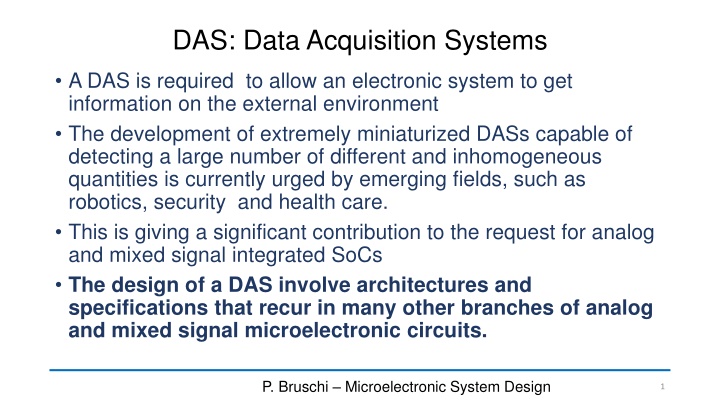
DAS: Data Acquisition Systems A DAS is required to allow an electronic system to get information on the external environment The development of extremely miniaturized DASs capable of detecting a large number of different and inhomogeneous quantities is currently urged by emerging fields, such as robotics, security and health care. This is giving a significant contribution to the request for analog and mixed signal integrated SoCs The design of a DAS involve architectures and specifications that recur in many other branches of analog and mixed signal microelectronic circuits. P. Bruschi Microelectronic System Design 1
The electronic system and the enviroment P. Bruschi Design of Mixed Signal Circuits 2
Main blocks of an Electronic System DAS (full acquisition operations) P. Bruschi Microelectronic System Design 3
Elements of a DAS: a two-channel case P. Bruschi Microelectronic System Design 4
Signal classification on the basis of quantization Magnitude Time digital signals discrete time discrete time analog signals continuous time P. Bruschi Microelectronic System Design 5
Errors on the ideal transfer function ( ) f X = Nominal (ideal) case: V Once V is known, X can be known exactly: ( ) X g V = ( ) g x f = 1 ( ) (inverse function) x ( ) f X ( ) X = Real case: ( ) X V V e ( ) f X = ideal V is the output error defined as: Videal V e V In an acquisition system, the error is not known in a deterministic way. To find the input quantity (X) we can only apply the inverse (g) of the nominal transfer function to the real output quantity (we do not know the real t.f.): ( ) ( ) g V ( ) ( ) X = = X g f X V Xmis the "measurement result" m e P. Bruschi Microelectronic System Design 6
RTI (Referred to Input) Error ( ) f X ( ) X = V V Property of Inverse Functions e 1 ( ) dV ( ) dx dg V df x X = m ( ) g 1 ( ) dV dg V df dX ( ) ( ) ( ) X ( ) ( ) ( ) X = g f X V X V = X g f X V e e m e 1 df dX = = RTI Error X X X V e m e P. Bruschi Microelectronic System Design 7
RTI Error: Equivalent block diagram for small errors If the first order approximation that we have seen holds, it is possible to use the following equivalent representation: Verification: ( f X = df dX df dX ) ( ) f X Then, the equivalent block behaves as the real block V X X e e 1 = since: X V Ideal block e e Equivalent representation of the real block ( ) f X V V e In this case, the dc value of Xeis the input offset Xeis the value of the input quantity X that nulls the output = if: (0) f 0 P. Bruschi Microelectronic System Design 8
System performance vs type of errors Offset Gain error Non-linearity errors System Static Accuracy Noise System Resolution Dynamic errors (finite response time) System response speed P. Bruschi Microelectronic System Design 9
Non-linearity errors Generally, the maximum non- linearity error in the whole range of the input quantity X is indicated in the specifications VX linear approximation If the non-linear curve is well reproducible, the non-linearity error can be compensated for by means of a non-linear estimator. actual curve VX* For random non-linearities, individual multi-point trimming is necessary. Xm X = e nl x X X m P. Bruschi Microelectronic System Design 10
The dynamic error is the difference between the present value and the final value Maximum residual difference (band) Dynamic errors "overshoot" Settling time tset: Time required to have the output voltage stay close to the final value within a given residual difference Ideal Typical settling specs: 1 % (low accuracy) 0.01 % (high accuracy) damped oscillation: "ringing" P. Bruschi Microelectronic System Design 11
Linear time and slew-rate time Slew-rate only (most of the transition time at least one stage is saturated) Linear-time only (all stages behave linearly) (for1 % error no-ringing) 1 0.99 X X s X s t m m t set B set s 3 dB r r r P. Bruschi Microelectronic System Design 12
Noise and resolution Samples in this range are compatible with both the X and X+ X input. Therefore, it is not guaranteed that a difference X can be recognized Minimum difference X that can be reliably detected: = = X resolution n pp x min P. Bruschi Microelectronic System Design 13
Noise: peak-to-peak, rms and standard deviation = = 2 2 n pp x Cf= crest factor n p x c x n rms f Xn-pp f max = = 2 n ( ) f df n rms x x S xn f min For gaussian noise 1 probability Interval Total interval width (xnp-p) Probability If we sample the noise xn, then the standard deviation of the samples is: 2 3 4 2 4 6 8 0.683 (68.3 %) 0.317 0.954 (95.4 %) 0.046 0.997 (99.7 %) 0.003 6.4 10 5 0.999936 (99.9936 %) ( ) 2 = = x x x X n n rms = 4 4 n pp x x Our choice: X rms P. Bruschi Microelectronic System Design 14
The Dynamic Range (DR) Signal range X FS X DR Xmax x generally is the resolution Xmax Xmin=XFS Full scale (excursion) Xmin P. Bruschi Microelectronic System Design 15
DR and maximum number of significant levels Xmax X FS X DR Number of distinguishable levels = DR The presence of noise cause a sort of quantization of the analog signal, at least in terms of usable levels XFS Fist level that the system can distinguish from Xmin Xmin x For a digital signal coded with n bits: Number of levels = 2n ( ) = ln ENOB DR For an analog signal: Effective Number Of Bits 2 P. Bruschi Microelectronic System Design 16


 Error")


")