Engineering Approach for Converting SRS Levels
Learn how to convert Shock Response Spectrum (SRS) levels from one amplification factor to another by synthesizing time histories using damped sinusoids. This method, crucial in aerospace applications, ensures accurate representation of pyrotechnic shock pulses. Utilize Matlab for practical implementation and optimization of new SRS specifications.

Download Presentation

Please find below an Image/Link to download the presentation.
The content on the website is provided AS IS for your information and personal use only. It may not be sold, licensed, or shared on other websites without obtaining consent from the author. If you encounter any issues during the download, it is possible that the publisher has removed the file from their server.
You are allowed to download the files provided on this website for personal or commercial use, subject to the condition that they are used lawfully. All files are the property of their respective owners.
The content on the website is provided AS IS for your information and personal use only. It may not be sold, licensed, or shared on other websites without obtaining consent from the author.
E N D
Presentation Transcript
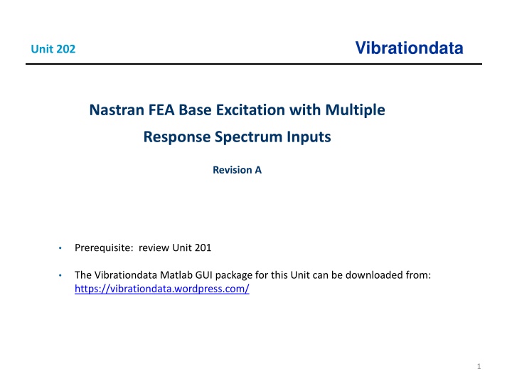
Vibrationdata Unit 202 Nastran FEA Base Excitation with Multiple Response Spectrum Inputs Revision A Prerequisite: review Unit 201 The Vibrationdata Matlab GUI package for this Unit can be downloaded from: https://vibrationdata.wordpress.com/ 1
Introduction Vibrationdata Aerospace pyrotechnic shock response spectrum (SRS) specifications are almost always given with an amplification factor Q=10 Corresponding time history waveforms for the base input acceleration are almost never given with the specifications Users are allowed to synthesize their own waveforms for analysis & test purposes Some shock analysis methods use the SRS directly without time history synthesis, such as modal combination methods Consider the following specification with Q=10 What should be the new SRS level for Q=20 or 50? SRS Q=10 fn (Hz) Peak Accel (G) Pyrotechnic SRS specifications typically begin at 100 Hz, but extrapolation down to 10 Hz may be needed if the structure has any modal frequencies below 100 Hz 10 10 2000 2000 10000 2000 2
Introduction Vibrationdata There is no exact way to convert an SRS to a new Q value unless a corresponding time history is included with the SRS The following is a reasonable approach for engineering purposes Synthesize a time history to satisfy the SRS using a series of damped sinusoids The resulting time history should resemble a pyrotechnic pulse or whatever pulse the SRS is suppose to represent Verify the synthesis with respect to the SRS with its original Q value Calculate the SRS of the synthesize signal with the new Q value The new SRS will be somewhat jagged Take the average or a maximum envelope of the jagged SRS to obtain a new smooth SRS specification, using trial-and-error curve-fitting to minimize the difference An example using Matlab is shown on the following slides 3
SRS Conversion Function >> spec = [10 10; 2000 2000; 10000 2000] 5
Synthesized Time History The time history is a series of damped sinusoids It is a plausible representation of a pyrotechnic shock pulse 6
Synthesized Time History Verification The positive & negative curves are from the synthesized time history The time history satisfies the specification within reasonable tolerance bands 7
New Specification Q=20 The jagged lines are the SRS of the synthesized time history The new spec is a ramp-plateau average which seeks to minimize the difference with respect to the absolute value SRS of the synthesis 8
New Specification Q=50 The jagged lines are the SRS of the synthesized time history The new spec is a ramp-plateau average which seeks to minimize the difference with respect to the absolute value SRS of the synthesis 9
SRS Specifications for Two Q Values The new spec can be used for analyzing the response of a single-degree-of-freedom system with Q=20 or 50 Interpolation can be used for other Q values between Q=10 and Q=50 The curves can also be used for multi-degree-of-freedom systems via modal combination methods 10
SRS Specification Comparison Vibrationdata Old Spec New Spec 1 New Spec 2 SRS Q=10 SRS Q=20 SRS Q=50 fn (Hz) Peak Accel (G) fn (Hz) Peak Accel (G) fn (Hz) Peak Accel (G) 10 13.52 10 10 10 12.2 1709 3587 2000 2000 1784 2633 10000 3587 10000 2000 10000 2633 Output arrays: synthesized_acceleration synthesized_srs_old_Q srs_spec_new_Q20 srs_spec_new_Q50 11
Spec is the SRS with Q=10 Choose Function Number 7 Export as: SRS_Q10.bdf 13
Choose Function Number 8 Export as: SRS_Q20.bdf 14
Choose Function Number 9 Export as: SRS_Q50.bdf 15
Introduction Vibrationdata Shock and vibration analysis can be performed either in the frequency or time domain Continue with plate from Units 200 & 201 Aluminum, 12 x 12 x 0.25 inch Rigid links Translation constrained at corner nodes Mount plate to heavy seismic mass via rigid links Use response spectrum analysis SRS is shock response spectrum Delete all output and all functions if you are reusing Unit 201 model The following software steps must be followed carefully, otherwise errors will result 16
Procedure, part I Vibrationdata Femap, NX Nastran and the Vibrationdata Matlab GUI package are all used in this analysis The GUI package can be downloaded from: https://vibrationdata.wordpress.com/ Recall the plate center node 1201 Parameters for T3 Modal Mass Fraction Participation Factor n fn (Hz) Eigenvector 1 117.6 0.933 0.0923 13.98 6 723.6 0.036 0.0182 22.28 12 1502 0.017 0.0123 2.499 19 2266 0.003 0.0053 32.22 The Participation Factors & Eigenvectors are shown as absolute values The Eigenvectors are mass-normalized Modes 1, 6, 12 & 19 account for 98.9% of the total mass 17
Femap: Seismic Constraints The four plate corner nodes are constrained in T1 & T2 The lower nodes are constrained in all but T3 18
Femap: Kinematic Constraint Constrain TZ The seismic mass is constrained in TZ which is the response spectrum base drive axis 19
Femap: Define Q Damping Function Q Damping varies between 0 and 4000 Hz 20
Femap: Q Values by Mode Number n fn (Hz) Q 11.2 1 117.6 17.2 6 723.6 25.0 12 1502 32.7 19 2266 Nastran will perform interpolation for each mode using the three SRS curves in the following slides 21
Femap: Import SRS Q=10 Function (cont) Change title to SRS Q=10 23
Femap: Import SRS Q=20 Function Change title to SRS Q=20 24
Femap: Import SRS Q=50 Function Change title to SRS Q=50 25
Femap: Analysis Each imported SRS function will add an Analysis function Delete all of these extra Analysis cases 26
Femap: Define Function vs. Critical Damping for Cross-reference Function Q Damping Ratio Nastran will perform interpolation for each mode using the three SRS functions 7 10 0.05 8 20 0.025 19 50 0.01 27
Femap: Define Normal Modes Analysis with Response Spectrum 28
Femap: Define Normal Modes Analysis Parameters Solve for 20 modes 29
Femap: SRS Cross-Reference Function This is the function that relates the SRS specifications to their respective damping cases Square root of the sum of the squares The responses from modes with closely-spaced frequencies will be lumped together 31
Femap: Define Boundary Conditions Main Constraint function Base input constraint, TZ for this example 32
Femap: Define Outputs Quick and easy to output results at all nodes & elements for response spectrum analysis Only subset of nodes & elements was output for modal transient analysis due to file size and processing time considerations Get output f06 file 33
Femap: Export Nastran Analysis File Export analysis file Run in Nastran 34
Matlab: Response Spectrum Results Maximum Displacements: node value T1: 2376 0.00000 in T2: 931 0.00000 in T3: 1201 0.17744 in R1: 1 0.03397 rad/sec R2: 1 0.03397 rad/sec R3: 1 0.00000 rad/sec Maximum accelerations: node value T1: 2376 0.000 G T2: 931 0.000 G T3: 49 1237.766 G R1: 1 236412.400 rad/sec^2 R2: 1 236412.400 rad/sec^2 R3: 1 0.000 rad/sec^2 Maximum Quad4 Stress: element value NORMAL-X : 1105 10082.950 psi NORMAL-Y : 24 10082.950 psi SHEAR-XY : 50 8072.997 psi MAJOR PRNCPL: 50 10172.070 psi MINOR PRNCPL: 1128 8426.593 psi VON MISES : 50 14139.520 psi Maximum velocities: node value T1: 2376 0.000 in/sec T2: 931 0.000 in/sec T3: 1201 140.588 in/sec R1: 2354 36.947 rad/sec R2: 1 36.947 rad/sec R3: 1 0.000 rad/sec 38
Matlab: Response Spectrum Acceleration Results (cont) Node 49 Node 1201 Center node 1201 had T3 peak acceleration = 874.9 G Edge node 49 had highest T3 peak acceleration = 1238 G By symmetry, three other edge nodes should have this same acceleration But node 1201 had highest displacement and velocity responses 39
Femap: T3 Acceleration Contour Plot, unit = in/sec^2 Import the f06 file into Femap and then View > Select 40
Procedure, part II Response spectrum analysis is actually an extension of normal modes analysis ABSSUM absolute sum method SRSS square-root-of-the-sum-of-the-squares NRL Naval Research Laboratory method The SRSS method is probably the best choice for response spectrum analysis because the modal oscillators tend to reach their respective peaks at different times according to frequency The lower natural frequency oscillators take longer to peak 42
ABSSUM Method Conservative assumption that all modal peaks occur simultaneously N ( ) = j q i z j i j max max 1 Pick D values directly off of Relative Displacement SRS curve N = ( ) q iz D max j j i , j max j 1 where is the mass-normalized eigenvector coefficient for coordinate i and mode j j i q These equations are valid for both relative displacement and absolute acceleration. 43
SRSS Method N ( ) 2 = j q iz j i , j max max 1 Pick D values directly off of Relative Displacement SRS curve N ( ) 2 = j q iz D j j i , j max max 1 These equations are valid for both relative displacement and absolute acceleration. 44
SRS Curve Interpolation Q=10 SRS (G) Q=20 SRS (G) Q=50 SRS (G) Interpolated SRS (G) fn (Hz) n Q 1 117.6 11.2 117.6 157.1 196.2 122.3 6 723.6 17.2 723.6 1033 1411 946.4 12 1502 25.0 1502 2203 3118 2356 19 2266 32.7 2000 2633 3587 3037 The last column is the interpolated SRS for the given fn and Q values. 45
Acceleration Response Check for Node 1201 T3 | PF x Eig x Spec |2 (G2) Eigen vector Interpolated SRS (G) | PF x Eig x Spec | (G) fn (Hz) n Q PF 1 117.6 11.2 122.3 157.8 24904 0.0923 13.98 6 723.6 17.2 946.4 383.8 147273 0.0182 -22.28 12 1502 25.0 2356 72.4 5244 0.0123 2.499 19 2266 32.7 3037 518.6 268963 0.0053 32.22 sum = 446,384 G2 sum = 1133 G sqrt of sum = 668 G The table is taken from the plate model modal analysis results prior to the addition of the seismic mass, with three added columns The set composed of modes 1, 6, 12 & 19 accounts for almost 99% of the total mass The seventh column is the participation factor times the eigenvector times the SRS specification The sum of the absolute responses is 1133 G, which conservatively assumes that each mode reaches its peak at the same time as the others The square root of the sum of the squares is 668 G The FEA modal peak response was 874.9 G which passes the sanity check 46
Vibrationdata MDOF SRS with Variable Q Results fn Q=10 Q=20 Q=50 (Hz) SRS(G) SRS(G) SRS(G) 117.6 117.6 723.6 723.6 1502 1502 2266 2000 fn Part Eigen SRS Modal Response (Hz) Factor vector Accel(G) Accel(G) 117.6 0.0923 13.98 723.6 0.0182 -22.28 1502 0.0123 2.499 2266 0.0053 32.2 157.1 196.3 1033 2203 3118 2633 3587 1411 122.3 946.5 2355 3037 157.9 383.8 72.4 518.3 ABSSUM= 1132 G SRSS= 667.9 G Again, The FEA modal peak response was 874.9 G which passes the sanity check 50


")


")