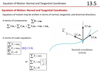
Equations of Motion in Local Cartesian Reference Frame
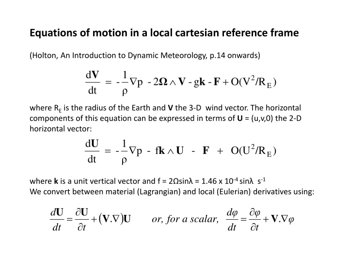
In meteorology, understanding the dynamics of wind flow is crucial. This equation describes the motion in a local Cartesian reference frame, considering factors such as gravitational acceleration and Coriolis force. It provides a mathematical framework to study atmospheric dynamics and predict weather patterns. With Earth's radius and wind vector as variables, this equation helps meteorologists analyze and model the complex behaviors of the atmosphere. By solving these equations, scientists gain insights into the intricate interactions that shape our weather systems.

Download Presentation

Please find below an Image/Link to download the presentation.
The content on the website is provided AS IS for your information and personal use only. It may not be sold, licensed, or shared on other websites without obtaining consent from the author.If you encounter any issues during the download, it is possible that the publisher has removed the file from their server.
You are allowed to download the files provided on this website for personal or commercial use, subject to the condition that they are used lawfully. All files are the property of their respective owners.
The content on the website is provided AS IS for your information and personal use only. It may not be sold, licensed, or shared on other websites without obtaining consent from the author.
E N D
Presentation Transcript
Equations of motion in a local cartesian reference frame (Holton, An Introduction to Dynamic Meteorology, p.14 onwards) V d 1 2 - = - O(V + g - V k F 2 - p /R ) E dt where RE is the radius of the Earth and V the 3-D wind vector. The horizontal components of this equation can be expressed in terms of U = (u,v,0) the 2-D horizontal vector: 1 - dt U d 2 = - O(U + k U F f - p /R ) E where k is a unit vertical vector and f = 2 sin = 1.46 x 10⁻⁴ sin s-1 We convert between material (Lagrangian) and local (Eulerian) derivatives using: U U d d ( ) = + . = + . V U V or, scalar, a for dt t dt t
In component form the full equations are: + + x dt du 1 p uv uw = - fv - F - 2 - E w cos tan x R R E 2 dv 1 p u vw = + - - y fu - F - y tan dt R R E E 2 2 + dw 1 p u v = + + - - z - g F 2 u cos z dt R E
Scale analysis For the synoptic-scale motions that we are interested in Horizontal scale L ~ 106 m Vertical scale D ~ 104 m Time scale T ~ 105 s Typical horizontal wind U ~ 10 ms-1 Typical vertical wind w~ 0.01 ms-1 Pressure p ~ 105 Pa (1000 mb) Typical pressure excursion p ~ 30 mb = 3000 Pa horizontally Surface air density ~ 1 kg m-3 Radius of Earth RE ~ 107 m Earth rotation rate ~ 10-4 s-1
Scale analysis: vertical momentum equation Horizontal scale L ~ 106 m Vertical scale D ~ 104 m Time scale T ~ 105 s Typical horizontal wind U ~ 10 ms-1 Typical vertical wind w~ 0.01 ms-1 Pressure p ~ 105 Pa (1000 mb) Typical pressure excursion p ~ 30 mb = 3000 Pa horizontally Surface air density ~ 1 kg m-3 Radius of Earth RE ~ 107 m Earth rotation rate ~ 10-4 s-1 2 2 + dw 1 p u v = + + - - z - g F 2 u cos z dt R E W/T p/D g U2/RE U 10-7 10 10 10-5 10-3
Scale analysis: horizontal momentum equation Horizontal scale L ~ 106 m Vertical scale D ~ 104 m Time scale T ~ 105 s Typical horizontal wind U ~ 10 ms-1 Typical vertical wind w~ 0.01 ms-1 Pressure p ~ 105 Pa (1000 mb) Typical pressure excursion p ~ 30 mb = 3000 Pa horizontally Surface air density ~ 1 kg m-3 Radius of Earth RE ~ 107 m Earth rotation rate ~ 10-4 s-1 U d 1 - = - O(1/R + k U F f - p ) E dt U/T p/L fU U2/RE 10-4 10-3 10-3 10-5