Equilibria in Material Systems: Laws of Thermodynamics

MSEG 803 Equilibria in Material Systems 3: Second Law of TD Prof. Juejun (JJ) Hu hujuejun@udel.edu

Generalized first law of TD Energy is conserved! + = + = dU Q W Q y dx i i i intensive extensive Can all processes that obey the law of energy conservation proceed spontaneously?

Perpetual motion machines of the 1st kind Produce work without input of energy Over 600 patents on perpetual motion machines were granted from 1635 to 1903 in UK only! Some examples of perpetual motion machines

Perpetual motion machines of the 2nd kind Spontaneously converts heat into work Hout (ice) Hwater-ice = 2261 J/g To produce 1 hp of power, 746 2261 / / dm dt kJ s J g work = = 330 / g s Only 330 g of water needs to be turned into ice per second! Hin (water)

Entropy S Extensive state function S(U, V, N, ) or S(U1, U2, , V1, V2, , N1, N2, ) for a composite system 1 T S U = 0 Monotonically increases with U, i.e. V N , ,... Q and satisfies the relation: dS sys T sys where the equality holds only in reversible processes The function S has the following property: the values assumed by the extensive parameters in the absence of an internal constraint are those that maximize S over the manifold of constrained equilibrium states.

Entropy S Microscopically, entropy S is a measure of the degree of disorder (# of accessible microscopic states) in a system An isolated system can spontaneously evolves into a state of higher degree of disorder but not vice versa

Directionality (reversibility) of processes State A State B Q A B: A B dS A B T Q T Q B A: = = A B B A dS dS B A A B T Q B A dS B A T Q = Reversible only when A B dS A B T

Process reversibility dS = 0 in an isolated/closed system Isolated system: one that cannot exchange energy in the form of heat or work with any other system, i.e. (U = constant) dS > 0 in irreversible processes Reversibility requires the system to be in equilibrium with environment at all times (zero driving force), i.e. reversible processes have to be quasi-static A quasi-static process, however, is not necessarily reversible Friction

Process reversibility (contd) Reif 3.2: Consider an isolated system which evolves from an initial state to a final state due to removal of an internal constraint If imposing the constraint on the final state can restore the initial state, then the process is reversible If the initial state cannot be restored even with imposition of the constraint, the process is irreversible Reversibility is a property of a process not a system

Final state : P1 = P2 Driving force: P1 - P2 P1 > P2 : dV change is irreversible P1 = P2 : dV change is reversible T, P1 T, P2 Constraint with respect to volume Final state : T1 = T2 Driving force: T2 - T1 T2 > T1 : Q change is irreversible T2 = T1 : Q change is reversible T1, P T2, P Adiabatic partition: constraint with respect to heat flow Final state : CA,1 = CA,2; CB,1 = CB,2 Driving force: concentration gradient dNA and dNB : irreversible Molecule A Molecule B Impermeable partition: constraint with respect to molecular flow

A cylinder of gas separated by a piston which has (arbitrarily) low thermal conductance. As the thermal conductance is low, at any given time, gas in each side of the cylinder can be described by a set T1, P1, V1 T2, P2, V2 of state functions Ti, Pi, Vi (i = 1, 2). A small heat transfer Q occurs between the two parts of gas. Is this a reversible process? T Q = dS T T Entropy change of sub-system 1: 1 1 2 1 T T Q = dS Entropy change of sub-system 2: 2 2 T Q Q = + = 0 dS dS dS Total entropy change: 1 2 1 2 Thus the process is irreversible (nor a quasi-static process as the driving force, i.e. temperature difference is not zero).

Properties of entropy S = ( ) sub sys S S Additive: S is an extensive state function s(u, v) = S(U, V, N)/N : molar entropy (intensive) S(U, V, N) = S( U, V, N), where is a constant (S is a homogeneous first order function of the extensive variables) S of a system is path independent S is not conserved Example: converting work to heat (Joule experiment) S of an open system can decrease at the expense of entropy increase of another system sys Q = + 0 dS dS dS System Environment t t o sys env Q T = Q T + / / dS dS sys sys env sys

Colloidal crystals: an example of self- assembled structures Ph.D. thesis, Lindsey Brooks Jerrim Stamm, North Carolina State University (2009).

Deriving equilibrium conditions In an isolated system, S always maximizes at equilibrium over the set of thermodynamic states consistent with the constraints (the manifold of constrained TD states) Equilibrium is attained through re-distribution of some unconstrained extensive parameters Equilibrium is reached if: 1) the conjugate intensive parameter ( potential ) of the unconstrained extensive parameter becomes uniform in the system; 2) dS = 0 when the unconstrained extensive parameter is re- distributed by an infinitesimal amount

Deriving equilibrium conditions equilibrium state S S xk S(xk) when xi = xi0 Constraint: xi = xi0 Unconstrained parameter: xk At equilibrium, xk assumes the value where S is maximum, i.e. dS = 0 when xk is changed by an infinitesimal amount dxk S x xk xi = xi0 (e.g. U1) 2 xi(e.g. V1) S = 0 0 2 x k k x x i i

Deriving equilibrium conditions Solving equilibrium condition in a composite system after removal of internal constraints Apply dS = 0 (maximizing S) under given constraints Example 1: equilibrium in an isolated system after removal of an adiabatic partition (i.e. only allows heat flow between sub-systems) T1 T2 = = + Q Q U U U is a constant Constraint: 2 1 1 2 tot 1 T 1 T Q T Q T = + = + = = ( ) 0 1 2 dS dS dS Q Apply dS = 0: 1 2 1 tot 1 2 1 2 = T T thermal equilibrium 1 2

Example 2: equilibrium in an isolated system after removal of an adiabatic, rigid partition (i.e. allows both heat flow and volume change of sub-systems) T1, V1 T2, V2 = = + dU dU U U U is a constant Constraint 1: 1 + 2 2 1 tot = = V V V dV dV is a constant Constraint 2: 1 2 2 1 tot Apply dS = 0: S U S U S V S V = + + + 1 2 1 2 dS dU dU dV dV 1 2 1 2 tot V N V N U N 1 2 1 2 , , , , U N 1 1 2 2 1 1 2 2 1 T S U S V P T 1 T 1 T P T P T = = = = 1 2 and V N U N , , 2 2 2 2 = = T T P P thermal equilibrium mechanical equilibrium 1 2 1 2

Example 3: equilibrium in an isolated system after removal of a rigid partition (i.e. allows only volume change of sub- systems) T1, V1 T2, V2 = + = U U U W W is a constant Constraint 1: 1 2 2 1 tot = + = dV dV V V V is a constant Constraint 2: 1 2 2 1 tot 1 T S U S V P T = = = P P V N U N 1 2 , , mechanical equilibrium Apply dS = 0: S U S U S V S V = + + + 1 2 1 2 dS dU dU dV dV 1 2 1 2 tot V N V N U N 1 2 1 2 , , , , U N 1 1 2 2 1 1 2 2 1 T 1 T P T P T = + 0 1 2 W W dV dV Indeterminate problem 1 2 1 2 1 2 1 2

Q Re-examining dS sys T sys In an irreversible process: Q dS T = + dissipation Dissipation: loss of useful work To calculate entropy change of a system in an irreversible process, a reversible process can usually be constructed which brings the system under investigation from the same initial state to end state as the irreversible process does

Example: Joules experiment Enclosed by an adiabatic wall Mechanical work W Water (system) Water (system) Conversion of work to heat Q = 0, U > 0 Entropy change of water S > 0 as A reversible process can be constructed by successively bringing the system (water) into contact with a series of heat reservoirs T T water T 1 T S U = 0 V N , ,... ( ) T C T Q T + = = 0 S dT P

Example: free expansion of ideal gas Initial state A Ideal gas Vacuum PV = constant = T T End state B A B C Ideal gas C T C T T T = + = + = + C B C C R V S S S dT dT P P V AB AC CB T T A C C T T T C T P P R T Q T T T T = = = = = C C C ln( ) ln( ) 0 V C dT dT dT R R P A T T T A A A A C

The maximum work theorem For all processes leading from the specified initial state to the specified final state of the primary system, the delivery of work is maximum for a reversible process = 0 W dU Q Q T Heat sys reservoir at T = 0 dS dS Q tot sys Q TdS sys W System W dU TdS sys sys W dU TdS sys sys State A B: dU

Heat engine 0 Q 0, W = = 0 dU dU sys Heat reservoir at T = = W dU Q Q sys Q = = 0 dS dS sys W Q T Q T System = = 0 dS dS tot sys State A A: dU = 0 Kelvin s formulation of the 2nd law of TD: it is impossible to construct a perfect heat engine which converts heat to work with 100% efficiency The system has to restore its initial state for sustainable output

Heat engine (contd) 0 Q 0, Q 0, W 2 1 Hot heat reservoir at T1 T T 1 2 = W Q Q 1 2 Q1 Q T Q T = + 1 2 0 dS dS tot sys W 1 2 System T T 2 Q Q 2 1 1 T T Q2 (1 ) 2 W Q 1 1 Cold heat reservoir at T2 W Q T T Engine efficiency = 1 2 1 1 State A A: dU = 0

Carnot cycle A to B (isothermal expansion): dT = 0, Q > 0, dS > 0, W < 0 B to C (adiabatic expansion): dT < 0, Q = 0, dS = 0, W < 0 C to D (isothermal compression): dT = 0, Q < 0, dS < 0, W > 0 D to A (adiabatic compression): dT > 0, Q = 0, dS = 0, W > 0

Other reversible heat engine cycles Otto cycle Joule cycle All reversible heat engine cycles have the same efficiency!

Heat pump Transfers heat from a low temperature reservoir to a high temperature reservoir Heat pump coefficient of performance: Q W T Q W T Hot heat reservoir at T1 T T 1 2 Q1 W System T T = 2 2 for cooling T 1 2 Q2 = 1 1 for heating T Cold heat reservoir at T2 1 2 Can be greater than unity! State A A: dU = 0

Practical heat engine design: Rankine cycle Working substance: liquid rather than gas Ease of transporting liquid through the system Turbine Condenser Boiler

Practical heat engine design: Rankine cycle Working substance: liquid rather than gas Ease of transporting liquid through the system

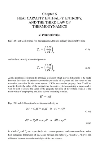
Entropy of materials When phase change is not involved: S ( ) Q constr C T = = ( ) constr dS dT constr T slope: Cliquid /T S T S T step: Hfus /Tm = = C T C T P V P V slope: Csolid /T When phase change is involved: ( ) ( ) constr dS T 0 T Q dH = = constr constr T

The 3rd law of thermodynamics The entropy of any TD system vanishes (S 0) in as temperature approaches absolute zero The change of entropy S 0 in any reversible isothermal process at T 0K (Nernst statement) Heat capacity C 0 as T 0K dT S T C T T T = ( ) ( ) is a finite number! 0 In classical thermodynamics, the absolute value of S has no physical significance S 0 can only be derived by statistical mechanics

Unattainability of absolute zero We cannot achieve absolute zero by heat transfer alone W < 0, dU < 0: the only way to reduce T is to let the system perform work through reversible processes S V = V2 > V1 (or x = x2 < x1) V = V1 (or any extensive function x = x1) http://ltl.tkk.fi/wiki/L TL/World_record_in _low_temperatures T 0