Essential Concepts in R Programming for Statistical Computing
"Learn about R programming language used for statistical computing, data analysis, and visualization. Explore variables, data structures like vectors and lists, and dive into fundamental concepts to enhance your programming skills."

Download Presentation

Please find below an Image/Link to download the presentation.
The content on the website is provided AS IS for your information and personal use only. It may not be sold, licensed, or shared on other websites without obtaining consent from the author. If you encounter any issues during the download, it is possible that the publisher has removed the file from their server.
You are allowed to download the files provided on this website for personal or commercial use, subject to the condition that they are used lawfully. All files are the property of their respective owners.
The content on the website is provided AS IS for your information and personal use only. It may not be sold, licensed, or shared on other websites without obtaining consent from the author.
E N D
Presentation Transcript
Programming with R Prepared by, MS.S.S.NACHIYA , M.C.A., M.Phil.,UGC-NET ASST. PROF. IN COMPUTER SCIENCE, SHRIMATI INDIRA GANDHI COLLEGE, TIRUCHIRAPPALLI - 2 1
Introduction R is a popular programming language used for statistical computing and graphical presentation. Its most common use is to analyze and visualize data. It is easy to draw graphs in R, like pie charts, histograms, box plot, scatter plot, etc++ It works on different platforms (Windows, Mac, Linux) It is open-source and free It has a large community support It has many packages (libraries of functions) that can be used to solve different problems. 2
R Variables A variable is a memory allocated for the storage of specific data and the name associated with the variable is used to work around this reserved block. Syntax Using equal to operators variable_name = value using leftward operator variable_name <- value using rightward operator value -> variable_name 3
Example # using equal to operator var1 = "hello" print(var1) # using leftward operator var2 <- "hello" print(var2) # using rightward operator "hello" -> var3 print(var3) Output [1] "hello" [1] "hello" [1] "hello" 4
Data Structures in R 5
The most essential data structures used in R include: Vectors Lists Dataframes Matrices Arrays Factors 6
Vectors Vector is one of the basic data structures in R. It is homogenous, which means that it only contains elements of the same data type. Data types can be numeric, integer, character, complex, or logical. Example # Vectors(ordered collection of same data type) X = c(1, 3, 5, 7, 8) # Printing those elements in console print(X) Output [1] 1 3 5 7 8 7
Lists A list is a non-homogeneous data structure, which implies that it can contain elements of different data types. It accepts numbers, characters, lists, and even matrices and functions inside it. It is created by using the list() function. Example empId = c(1, 2, 3, 4) empName = c("Debi", "Sandeep", "Subham", "Shiba") numberOfEmp = 4 empList = list(empId, empName, numberOfEmp) print(empList) Output [[1]] [1] 1 2 3 4 [[2]] [1] "Debi" "Sandeep" "Subham" "Shiba [[3]] [1] 4 8
Matrices A matrix is a rectangular arrangement of numbers in rows and columns. In a matrix, as we know rows are the ones that run horizontally and columns are the ones that run vertically. Matrices are two-dimensional, homogeneous data structures. Example M1 <- matrix(c(1:9), nrow = 3, ncol =3, byrow= TRUE) print(M1) Output [,1] [,2] [,3] [,1] 1 2 3 [,2] 4 5 6 [,3] 7 8 9 9
Arrays items of a similar type together. This leads to a collection of items that are stored at contiguous memory locations. This memory location is denoted by the array name. The position of an element can be calculated simply by adding an offset to its base value. Example Array Structure An array consists of the following: Array Index: The array index identifies the location of the element. The array index starts with 0. Array Element: Array elements are items that are stored in the array. Array Length: The array length is determined by the number of elements that can be stored by the array. . Arrays refer to the type of data structure that is used to store multiple 10
There are two types of arrays: One-dimensional Arrays Multi-dimensional Arrays One-dimensional Arrays One- or single-dimensional arrays are the types of arrays that have array elements stored in a sequence and can be accessed in the same order. Multi-dimensional Arrays Multi-dimensional arrays are arrays that have elements stored in more than one dimension. They can be two- or three-dimensional arrays and can consist of row and column indexes. To create an array in R: The array() function is utilised. In this function, the input is a vector. For creating the array, the value in the dim parameter is utilised. 11
For example: In this following example, we will create an array in R of two 3 3 matrices each with 3 rows and 3 columns. # Create two vectors of different lengths. > vec1 <- c(1,2,4) #Author DataFlair > vec2 <- c(15,17,27,3,10,11) > output <- array(c(vec1,vec2),dim = c(3,3,2)) 12
Output 13
Data Frames A data frame is a two-dimensional array-like structure, or we can say it is a table in which each column contains the value of one variable, and row contains the set of value from each column. There are the following characteristics of a data frame: The column name will be non-empty. The row names will be unique. A data frame stored numeric, factor or character type data. Each column will contain same number of data items. To create a data frame we use the data.frame() function. 14
R program to illustrate dataframe # A vector which is a character vector Name = c("Amiya", "Raj", "Asish") # A vector which is a character vector Language = c("R", "Python", "Java") # A vector which is a numeric vector Age = c(22, 25, 45) # To create dataframe use data.frame command # and then pass each of the vectors # we have created as arguments # to the function data.frame() df = data.frame(Name, Language, Age) print(df) 15
Output: Name Language Age 1 Amiya R 22 2 Raj Python 25 3 Asish Java 45 16
Factors and store it as levels. Factors can store both strings and integers. Columns have a limited number of unique values so that factors are very useful in columns. It is very useful in data analysis for statistical modeling. Factors are also data objects that are used to categorize the data Factors are created with the help of factor() function by taking a vector as an input parameter. 17
Example # Create a vector as input. data<- ("East","West","East","North","North","East","West","West","West","East","North") print(data) print(is.factor(data)) # Apply the factor function. factor_data <- factor(data) print(factor_data) print(is.factor(factor_data)) 18
Output [1] "East" "West" "East" "North" "North" "East" "West" "West" "West" "East" "North" [1] FALSE [1] East West East North North East West West West East North Levels: East North West [1] TRUE 19
Strings in R A string is a sequence of characters. For example, "Programming" is a string that includes characters: P, r, o, g, r, a, m, m, i, n, g. In R, we represent strings using quotation marks (double quotes, " " or single quotes, ' '). For example # string value using single quotes 'Hello # string value using double quotes "Hello" Example: Strings in R message1 <- 'Hola Amigos' print(message1) message2 <- "Welcome to Programiz" print(message2) Output [1] "Hola Amigos [1] "Welcome to Programiz" 20
Example a <- 'Start and end with single quote' print(a) b <- "Start and end with double quotes" print(b) c <- "single quote ' in between double quotes" print(c) d <- 'Double quotes " in between single quote' print(d) Output [1] Start and end with single quote [1] "Start and end with double quotes [1] "single quote ' in between double quote" [1] Double quote " in between single quote" 21
Join Strings Together In R, we can use the paste() function to join two or more strings together. For example message1 <- "Programiz" message2 <- "Pro" # use paste() to join two strings paste(message1, message2) Output [1] Programiz Pro Example message1 <- "Hello, World!" message2 <- "Hola, Mundo! message3 <- "Hello, World! # compare message1 and message2 print(message1 == message2) # compare message1 and message3 print(message1 == message3) Output [1] FALSE [1] TRUE 22
R Looping Loops are used to repeat the process until the expression (condition) is TRUE. R uses three keywords for, while and repeat for looping purpose. Next and break, provide additional control over the loop. The break statement exits the control from the innermost loop. The next statement immediately transfers control to return to the start of the loop and statement after next is skipped. The value returned by a loop statement is always NULL and is returned invisibly. 23
For Loop in R It is a type of control statement that enables one to easily construct an R loop that has to run statements or a set of statements multiple times. For R loop is commonly used to iterate over items of a sequence. It is an entry-controlled loop, in this loop, the test condition is tested first, then the body of the loop is executed, the loop body would not be executed if the test condition is false. Syntax: for (initialization_Statement; test_Expression; update_Statement) { // statements inside the body of the loop } 24
Example 1: Program to display numbers from 1 to 5 using for loop in R fruits<-list("apple","banana","cherry") for(x in fruits) { print(x) } Output [1] apple [1] banana [1] cherry anana" [1] "cherry [1]{ [1] [1] "apple[1] "apple" 26
While Loop in R It is a type of control statement that will run a statement or a set of statements repeatedly unless the given condition becomes false. It is also an entry-controlled loop, in this loop, the test condition is tested first, then the body of the loop is executed, the loop body would not be executed if the test condition is false. Syntax: while (expression) { statement } 27
Example: Print i as long as i is less than 6 i <- 1 while (i < 6) { print(i) i <- i + 1 } Output [ 1[[ [1] 1 [1] 2 [1] 3 [1] 4 [1] 5 [1] 4 29
Repeat loop A repeat loop is used to iterate a block of code. It is a special type of loop in which there is no condition to exit from the loop. For exiting, we include a break statement with a user-defined condition. This property of the loop makes it different from the other loops. A repeat loop constructs with the help of the repeat keyword in R. It is very easy to construct an infinite loop in R. Syntax: repeat { commands if(condition) { break } } 30
Example v <- c("Hello","repeat","loop") cnt <- 2 repeat { print(v) cnt <- cnt+1 if(cnt > 5) { break } } 32
Output: [1] Hello repeat loop [1] Hello repeat loop [1] Hello repeat loop [1] Hello repeat loop 33
Packages in R R packages are a collection of R functions, complied code and sample data. They are stored under a directory called "library" in the R environment. By default, R installs a set of packages during installation. More packages are added later, when they are needed for some specific purpose. When we start the R console, only the default packages are available by default. Other packages which are already installed have to be loaded explicitly to be used by the R program that is going to use them. 34
Loading packages in R For loading a package which is already existing and installed on your system, you can make use of and call the library function. Example >library() To execute the above code snippet will produce the following result 35
Get all packages currently loaded in the R environment >search() To execute the above code will produce the following result [1] ".GlobalEnv" "package:stats" "package:graphics" [4] "package:grDevices" "package:utils" "package:datasets" [7] "package:methods" "Autoloads" "package:base" Install a New Package There are two ways to add new R packages. One is installing directly from the CRAN directory and another is downloading the package to your local system and installing it manually. Install directly from CRAN The following command gets the packages directly from CRAN webpage and installs the package in the R environment. install.packages("Package Name") # Install the package named "XML". install.packages("XML") 36
Install package manually Go to the link R Packages to download the package needed. Save the package as a .zip file in a suitable location in the local system. Now you can run the following command to install this package in the R environment. install.packages(file_name_with_path, repos = NULL, type = "source") # Install the package named "XML install.packages("E:/XML_3.98-1.3.zip", repos = NULL, type = "source") 37
Load Package to Library Before a package can be used in the code, it must be loaded to the current R environment. You also need to load a package that is already installed previously but not available in the current environment. A package is loaded using the following command >library("package Name", lib.loc = "path to library") # Load the package named "XML install.packages("E:/XML_3.98-1.3.zip", repos = NULL, type = "source") 38
Maintaining packages in R After your packages get installed and you frequently want to update them in order to have an up to date latest versions. This is possible using update.packages. By default, the function will remind you to update each package. update.packages (ask = FALSE) # this won't ask for package updating It may happen that you may want to delete any package. It is possible using the remove.packages(). Example: remove.packages("zoo") 39
Dates and Times in R Depending on what purposes we're using R for, we may want to deal with data containing dates and times. R Provides us various functions to deal with dates and times. Get Current System Date, and Time in R In R, we use Sys.Date(), Sys.time() to get the current date and time respectively based on the local system. For example # get current system date Sys.Date() # get current system time Sys.time() Output [1] "2022-07-11 [1] "2022-07-11 04:16:52 UTC" 40
Using R lubridate Package The lubridate package in R makes the extraction and manipulation of some parts of the date value more efficient. There are various functions under this package that can be used to deal with dates. But first, in order to access the lubridate package, we first need to import the package as: # access lubridate package library(lubridate) 1.Get Current Date Using R lubridate Package # access lubridate package library(lubridate) # get current date with time and timezone now() # Output: "2022-07-11 04: 34: 23 UTC" 41
2. Extraction Years, Months, and Days from Multiple Date Values in R In R, we use the year(), month(), and mday() function provided by the lubridate package to extract years, months, and days respectively from multiple date values. For example, # import lubridate package library(lubridate) dates <- c("2022-07-11", "2012-04-19", "2017-03-08") # extract years from dates year(dates) # extract months from dates month(dates) # extract days from dates mday(dates) 42
Output [1] 2022 2012 2017 [1] 7 4 3 [1] 11 19 8 Here, year(dates) - returns all years from dates i.e. 2022 2012 2017 month(dates) - returns all months from dates i.e. 7 4 3 mday(dates) - returns days from dates i.e 11 19 8 43
Files in R In the R programming language, we deal with large amounts of data by representing data in files. In this regard, we can perform certain operations to access data like creating files, reading files, renaming them, etc. Some different file operations in R are: Creation of files Writing to the files Reading data from a file Check the existing status of a file Renaming the existing files 44
Creation of a file Using file.create() function, a new file can be created from console or truncates if already exists. Syntax: file.create( ) # Create a file if (file.create("GFG.txt") print( Congrats! Your File Has been created. ) else print( unable to create ) Output :[1] "Congrats! Your File Has been created." 45
Writing to the files write.table() function in R programming is used to write an object to a file. Syntax: write.table(x, file) Parameters: x: indicates the object that has to be written into the file file: indicates the name of the file that has to be written Example # into the txt file write.table(x=toothgrowth[1:10,], CFG.TXT ) data=read.table( CFG.TXT ) 46 print(data) # printing data
Output Output len supp dose 1 4.2 VC 0.5 2 11.5 VC 0.5 3 7.3 VC 0.5 4 5.8 VC 0.5 5 6.4 VC 0.5 6 10.0 VC 0.5 7 11.2 VC 0.5 8 11.2 VC 0.5 9 5.2 VC 0.5 10 7.0 VC 0.5 47
Reading data from a file After the writing data onto a file, we need to read the information from the file using built-in function. We use the read.table() function to read the file s content that is passed as an argument. Syntax: read.table(file) Parameters: file: indicates the name of the file that has to be read Example # Reading txt file new.iris <- read.table(file = "GFG.txt") # Print print(new.iris) 48
Output X Sepal.Length Sepal.Width Petal.Length Petal.Width Species 1 1 5.1 3.5 1.4 2 2 4.9 3.0 1.4 3 3 4.7 3.2 1.3 4 4 4.6 3.1 1.5 5 5 5.0 3.6 1.4 6 6 5.4 3.9 1.7 7 7 4.6 3.4 1.4 8 8 5.0 3.4 1.5 0.2 9 9 4.4 2.9 1.4 10 10 4.9 3.1 1.5 0.2 0.2 0.2 0.2 0.2 0.4 0.3 setosa setosa setosa setosa setosa setosa setosa setosa setosa setosa 0.2 0.1 49
Check an existing file We can check the file if it exists or not within the current directory or on the mentioned path using the file.exists() function. We need to pass the file name, and if the file name is in existence, it returns TRUE. Otherwise, it returns FALSE. Syntax file.exists( file_name ) Example if (file.exists( CFG.TXT )) { print( Your file CFG.TXT Exist! ) } else 50