Evolution of CLIC DR RF System Design
Discover the development path of the CLIC DR RF system design from 2008 to the present, including the introduction of baseline and alternative options, addressing beam loading effects, RF system issues, and advancements in conceptual designs. Dive into the evolutionary journey that has shaped the current state of the CLIC DR RF system.

Download Presentation

Please find below an Image/Link to download the presentation.
The content on the website is provided AS IS for your information and personal use only. It may not be sold, licensed, or shared on other websites without obtaining consent from the author. If you encounter any issues during the download, it is possible that the publisher has removed the file from their server.
You are allowed to download the files provided on this website for personal or commercial use, subject to the condition that they are used lawfully. All files are the property of their respective owners.
The content on the website is provided AS IS for your information and personal use only. It may not be sold, licensed, or shared on other websites without obtaining consent from the author.
E N D
Presentation Transcript
CLIC DR RF system Baseline and Alternatives A.Grudiev 19/09/2014 Acknowledgements for useful discussions to: K.Akai, S.Belomestnykh, W.Hofle, E.Jensen
Outline Introduction Beam loading effect Baseline 1 GHz alternatives SC option Option with RF frequency mismatch Option with strong input power modulations 2 GHz alternatives (will not be presented in details due to lack of time) Summary
CLIC DR RF system design evolution 2008, CLIC08, (Oct. 2008), 2 GHz RF system issues were raised for the first time, recommendations were given, 1 GHz was proposed as possible alternative. 2009, ACE (May 2009), Issues were presented to ACE and partially addressed. ACE recommended to develop concept for RF system. 2010, ACE (Feb. 2010), progress was reported. CLIC meting (March 2010) 1 GHz RF system with 2 bunch trains adopted for CLIC baseline Real work on the DR RF system conceptual design started IWLC (Oct. 2010), new DR parameters were presented (more favorable for RF system), several options for conceptual design of 2 GHz RF system were presented 2011, New parameter set for the DR: even more favorable for RF Conceptual design for the baseline at 1 GHz and several alternatives at 1 and 2 GHz are proposed for the CDR. Baseline published in CLIC CDR, alternatives in CLIC-Note-879 Basically, nothing happened since CDR is published
CLIC DR parameters CLIC DR F. Antoniou and Y. Papaphilippou Last update on 18 Jan. 2011 RF frequency: f [GHz] 1 2 Circumference: C [m] 427.5 Energy : E [GeV] 2.86 1.28 x 10⁻⁴ Momentum compaction: p 4.1 x 10⁹ Bunch population: Ne Number of bunches: NB 312 Number of trains: NT 2 1 Energy loss per turn: eVA[MeV] 3.98 Energy spread in the bunch: E/E [%] 0.12 Bunch length: Z[mm] 1.8 1.6 RF voltage: VC[MV] 5.1 4.5 Calculated RF parameters Harmonic number: h 1426 2852 Synchronous phase : [o] (0oon crest) 38.7 27.8 Synchrotron frequency: fs[kHz] 3.45 4.58 Synchrotron motion: small amplitude harmonic oscillation in longitudinal phase space Energy acceptance: E/E [%] 2.34 1.01 Bucket length 2 Z [mm] 70 35
Specifications from RTML Specification on the bunch-to-bunch spacing variation along the train: 0.1 degree at 1 GHz corresponds to 280 fs; or 84 m; Specification on the bunch-to-bunch variation of the bunch length ( Z) along the train: RMS{ Z}/ Z < 2% These are very tight specs for the DR RF system itself to meet It is also a challenge for beam diagnostics in the DR to measure it. Isn t it? N.B. At the equilibrium, mean energy and the energy spread are the same for all bunches. Only the bunch spacing and the bunch length are significantly affected by the beam loading transient within each revolution period. It is the scope of this presentation to address this effect. Slow (compared to the revolution period) variations are outside of the scope of this presentation. Slow feedback system should take care of this.
Beam loading effect (1/3) 2GHz case 1GHz case Variation of the stored energy and rf voltage due to beam loading ( VC/VC << 1): IB TR TB t 2 V V U = = ; 2 C C U 2 R Q U V C VC 1GHz case d U U ( ) = = P P VC B B dt T B N T ( ) = VA B R U P P B B N h T 1 N N eV N = B e A B N h T Condition to keep RF voltage variation small in an RF system with constant input rf power: 2 N N eV V N ; 1 B e A C B U U 2 N h R Q T
Beam loading effect (2/3) Variation of the bunch phase due to rf voltage variation ( VC/VC << 1): 1 B V V Im{V} VB = + VC V1 2 VC V V = = tan 1 C 1 V2 1 C V C V V V 1 2 = = 2 C 2 tan C V C V 1 = + tan C B tan C V 1 V Re{V} = C cos sin VA C
Beam loading effect (3/3) Variation of the bunch length due to rf voltage variation ( E<< E): ~ S Z const E = = ; ~ sin E V E S C ( Z ) 4 Z 2 2 V V const C A ( ) 4 + C V = 3 2 2 4 Z 2 0 V V V Z Z C A C Z+ Z V 1 1 V = C Z 2 2 sin Z C
Baseline solution (basic parameter chose) 1. RF frequency is 1 GHz 2. It is designed in a way that the stored energy is so high that the RF voltage variation is kept small to minimize the transient effect on the beam phase to be below the specifications 3. ARES-type cavity developed for the KEK B-factory RF system is used after scaling from 0.5 to 1 GHz and some modifications b = 0.1 degree RMS correspond to 0.3 degree peak-to-peak variation VC/VC = bcos sin = 0.26 % U/U = 2 VC/VC = 0.52 % U = NbNeeVA(1-Nb/h)/NT = 0.318 J U = U/( U/U) = 0.318 / 0.0052 = 61.2 J; R/Q = VC2/2 U = 33.8
Baseline solution (cavity parameter chose) Proposed in 1993 by Shintake, cavities of this type (ARES-type utilizing TE015 mode in storage cavity) are used in KEK B-factory in both low and high energy rings. It is equipped with tuning and HOM damping features. Frequency: f[GHz] 0.509 Normalized shunt impedance (circuit): Rg/Q [ ] 7.4 Unloaded Q-factor: Q 110000 Aperture radius: r [mm] 80 Power range: Pg=Vg2/2Rg [MW] Nominal Maximum tested 0.15 0.45 Gap voltage range: Vg [MV] Nominal Maximum tested 0.5 0.866 ~2.5 m Kageyama et al, APAC98
Baseline solution (cavity parameter chose) Cavity scaling from 0.5 to 1 GHz 1 GHz cavity modification to reduce R/Q R/Q=V2/2 (Ua+Us) in ARES Us=9Ua R/Q ~ 1/f3 Q ~ v/s ~ f Storage Cavity Storage Cavity TE~0 2 10 0.5 1 GHz TE 015 A C TE015 Scaling Vg to keep EM field amplitude constant : Vg ~ f -1 Vg ~ f 0 Frequency: f[GHz] 0.509 1 1 (~f-3) x 1/8 Normalized shunt impedance (circuit): Rg/Q [ ] (~f0) 7.4 7.4 0.925 Unloaded Q-factor: Q (~f-1/2) (~f1) x 2 110000 78000 156000 Aperture radius: r [mm] 80 40 40 Gap voltage range: Vg [kV] Nominal Maximum tested 500 866 250 433 same 250 433 In our case, an intermediate modification of the cavity is chosen to have comfortable voltage per cavity Vg = 5100 kV / 16 = 319 kV and the reduced Rg/Q = 33.8 / 16 = 2.11
Baseline solution (final parameter table) No issues Constant input rf power matched to the average beam power and power loss in the cavity walls Only standard feedback system, for example, like in KEK-B LER Remaining (minor) R&D is the rf design of the modified ARES- type cavity with reduced R/Q of 2.1 . Parameters of CLIC DR rf system at 1 GHz (baseline) KEK-B LER Rf frequency [GHz] 1 0.509 Total stored energy [J] 61.2 106 Total R/Q: [ ] 33.8 148 Cavity voltage: Vg [kV] 319 500 Number of cavities 16 20 Rg/Q per Cavity: [ ] 2.1 7.4 Q-factor 120000 110000 Total wall loss power [MW] 3.2 3.1 Average beam power [MW] 0.6 4.5 Total rf power [MW] 3.8 7.6 Number of klystrons 8 10 Required klystron power [MW] > 0.5 > 0.8 Total length of the rf system [m] 16 x 2 = 32 20 x 2.5 = 50 Bunch phase modulation p-p [deg] 0.3 (train 22%) 3.5 (gap 5%) K.Akai, et.al, EPAC98
Alternative solutions (motivations) Alternative solutions at 1 GHz Improve efficiency Reduce size/cost Alternative solutions at 2 GHz No train interleaving after the DR Improve efficiency Reduce size/cost
Alternative solutions 1.1 (superconducting cavity at 1 GHz) Superconductive RF system will be more efficient but not smaller or cheaper. Two options : 1. Superconducting ARES-type cavity. Since it is beyond present state-of-the-art in the SC RF technology an extensive R&D and prototyping will be necessary. It is not considered further. 2. Elliptical cavity. An example, is SCC used in KEK-B HER. It is equipped with tuners and HOM dampers. Must be scaled and modified to reduce R/Q. Frequency: f[GHz] 0.509 Normalized shunt impedance (circuit): Rg/Q [ ] 46.5 Unloaded Q-factor: Q ~1e9 Aperture radius: r [mm] 110 Beam loading Power range: [MW] Nominal Maximum tested 0.25 0.4 Gap voltage range: Vg [MV] Nominal Maximum tested 1.5 2 ~3 m Stored energy range: Ug [J] Nominal Maximum tested 7.7- 13.7 Y. Morita et al, IPAC10
Alternative solutions 1.1 (superconducting cavity at 1 GHz) Parameters of CLIC DR rf system at 1 GHz (baseline) Alternative 1.1 Elliptical cavity. Must be scaled and modified to reduce R/Q. This is done in two steps similar to ARES-type cavity scaling and modification: 1. Scaling by frequency ratio and keeping the same EM field amplitude: V~1/f, U~1/f3. 2. Increasing aperture to reduce the R/Q from 46.5 to 0.94 but assuming that the stored energy is constant. This is the main issue for this alternative. It is not obvious that the solution exists Rf frequency [GHz] 1 Total stored energy [J] 61.2 Stored energy per cavity [J] 3.8 1.7 Number of cavities 16 36 Total R/Q: [ ] 33.8 Rg/Q per gap: [ ] 2.1 0.94 Gap voltage: Vg [kV] 319 142 Q-factor 120000 ~1e9 Total wall loss power [MW] 3.2 ~0 Average beam power [MW] 0.6 Total rf power [MW] 3.8 0.6 Number of klystrons 8 9 Required klystron power [MW] > 0.5 > 0.07 (IOT?) Total length of the rf system [m] 16 x 2 = 32 36 x 3 = 108
Alternative solutions 1.2 (mismatch of rf frequency and 1 GHz) 1. RF frequency is close to 1 GHz 2. It is designed in a way that the stored energy is intermediately high, so that the rf voltage variation is kept small to minimize the transient effect to be below the specifications for the bunch length only 3. The remaining variation of the bunch phase is above the specification but it is linear and is compensated by reducing the rf frequency VC 1 0.8 VA 0.6 0.4 0.2 0 d 2 d 2 N N Trf = + = ; 1 b b T T T dT T f dT -0.2 rf b rf b N N -0.4 b b -0.6 d 2 N -0.8 = b T f dT b -1 3.5 N 0 0.5 1 1.5 2 2.5 3 4 4.5 5 b 1 1 = = = dTb < Trf ns 1 ; but GHz 1 dT f b GHz 1 T rf
Alternative solutions 1.2 (mismatch of rf frequency and 1 GHz) Basic parameters chose based on the bunch length specs Alternative 1.2 Baseline Z/ Z = 2% RMS correspond to 6% degree peak-to-peak variation b = 0.1 degree RMS 0.3 degree peak-to-peak VC/VC = -2 Z/ Z sin2 = 2 6% sin238.7o = 4.7 % VC/VC = 0.26 % U/U = 2 VC/VC = 9.4 % U/U = 0.52 % U = NbNeeVA(1-Nb/h)/NT = 0.318 J U = 0.318 J U = U/( U/U) = 0.318 / 0.094 = 3.4 J; U = 61.2 J; R/Q = VC2/2 U = 608 R/Q = 33.8
Alternative solutions 1.2(parameter table) Parameters of CLIC DR rf system at 1 GHz (baseline) Alternative 1.2 rf system with rf frequency is slightly lower than bunch rep. frequency to correct the bunch spacing to be exactly 1 ns. This frequency mismatch is bunch intensity dependent Remaining R&D: 1. the cavity design (conventional) 2. Accommodate the MRP change 3. an MD to demonstrate this compensation in an existing ring. (unless it is already done ?) Advantages: 1. More efficient 2. More compact 3. Less expensive Rf frequency [GHz] 1 Total stored energy [J] 61.2 3.4 Total R/Q: [ ] 33.8 608 Gap voltage: Vg [kV] 319 319 Number of cavities 16 16 Rg/Q per gap: [ ] 2.1 38 Q-factor 120000 ~30000 Total wall loss power [MW] 3.2 ~0.7 Average beam power [MW] 0.6 Total rf power [MW] 3.8 1.3 Number of klystrons 8 4 Required klystron power [MW] > 0.5 > 0.35 Total length of the rf system [m] 16 x 2 = 32 16 x 1 = 16 Bunch phase modulation p-p [deg] uncompensated 0.3 5.5 Relative frequency mismatch f/(1GHz) 1e-4 Corresponding MRP ( =50m) shift [mm] 5
Alternative solutions 1.2 (mismatch of rf frequency and 1 GHz) Bunch phase variation due to second order effects 8 2 beam generator cavity Ql = 10700 bunch phase spread [degree] 7 1 6 0 5 -1 V [MV] 4 -2 3 0 50 100 150 bunch number 200 250 300 350 0.02 2 0.012o RMS bunch phase spread [degree] 0.01 1 0 Effective 0 3.28 3.3 3.32 3.34 3.36 3.38 3.4 3.42 -0.01 t/Trf 4 x 10 -0.02 -0.03 -0.04 0 50 100 150 bunch number 200 250 300 350
Alternative solutions 1.3 (Input RF power modulation at 1 GHz) 1. RF frequency is 1 GHz 2. It is designed in a way that the stored energy is low. 3. The variation of the RF voltage are compensated by the modulation of the input RF power which is matched not to the average beam power but to the peak beam power, like in a linac AN RF CAVITY FOR THE NLC DAMPING RINGS, R.A. Rimmer, et al., PAC01. NLC DR RF cavity parameters CLIC DR RF Frequency: f[GHz] 0.714 1 Rg /Q [ ] (~ f 0) 120 120 Unloaded Q-factor: Q0 (~ f -1/2) 25000 21000 Aperture radius: r [mm] (~ f -1) 31 22 Gap voltage: Vg [MV] (~ f -1) Nominal - 0.5 - 0.35 - The same voltage per cavity and so the same number cavities as for the baseline solution is assumed: 16.
Alternative solutions 1.3(parameter table) An rf system similar to the linac rf system with repetition rate equivalent to the revolution frequency. Strong input power modulations are essential This requires an RF power source with larger bandwidth ~1% which is OK. This requires more sophisticated fast feedback and/or feed-forward systems A lots of R&D culminating in building a prototype and testing it in a ring are probably necessary: Advantages: 1. Slightly more efficient 2. More compact 3. Maybe less expensive Parameters of CLIC DR rf system at 1 GHz (baseline) Alternative 1.3 Rf frequency [GHz] 1 Number of cavities 16 Gap voltage: Vg [kV] 319 Rg/Q per gap: [ ] 2.1 120 Total R/Q: [ ] 33.8 1920 Total stored energy [J] 61.2 1.1 Q-factor 120000 21000 Total wall loss power [MW] 3.2 0.3 Reflected power [MW] 0 0.4 Average beam power [MW] 0.6 Peak beam power [MW] 2.6 Total rf power [MW] 3.2+0.6=3.8 0.3+0.4+2.6=3.3 Number of klystrons 8 8 Required klystron power [MW] > 0.5 > 0.4 Total length of the rf system [m] 16 x 2 = 32 16 x 0.5 = 8
Alternative solutions 1.3 (transients) Klystron bandwidth: 0 Klystron bandwidth: Klystron bandwidth: 1% 4 4 4 Drive Pin Prefl P0 Matched to average beam power. Ql = 5570 No input power modulations. Drive Pin Prefl P0 Matched to peak beam power. Ql = 2080 Input power modulations. 3 3 3 P [MW] P [MW] P [MW] 2 2 2 1 1 1 0 0 0 7200 7400 7600 7800 8000 8200 8400 t/Trf 7200 7400 7600 7800 8000 8200 8400 t/Trf Ql = 2080 1.72 1.74 1.76 1.78 t/Trf 1.8 1.82 1.84 4 x 10 8 8 8 beam generator cavity beam generator cavity Ql = 2080 7 7 7 6 6 6 5 5 5 V [MV] V [MV] V [MV] 4 4 4 3 3 3 2 2 2 beam generator cavity 1 1 Ql = 5570 1 0 0 0 7200 7400 7600 7800 t/Trf 8000 8200 8400 7200 7400 7600 7800 t/Trf 8000 8200 8400 1.72 1.74 1.76 1.78 t/Trf 1.8 1.82 1.84 4 -3 -4 x 10 3x 10 x 10 bunch phase spread [degree] 10 4 bunch phase spread [degree] bunch phase spread [degree] 2 5 2 1 0 0 0 -5 -2 -1 -2 -10 -4 0 50 100 150 200 250 300 0 50 100 150 200 250 300 0 50 100 150 200 250 300 bunch number bunch number bunch number
2 GHz alternatives Huge advantage for all these alternatives is no train interleaving after the DR
Summary table 1 GHz 2 GHz, no train interleaving after DR Classical RF system based on the NC ARES-type cavities Baseline PRF = 3.8 MW; L = 32 m; Cavity design: OK Alternative 2.0 PRF = 5.9 MW; L = 48 m; Cavity design: ok? Classical RF system based on the SCC cavities Alternative 1.1 PRF = 0.6 MW; L = 108 m; Cavity design: ok? Alternative 2.1 PRF = 0.6 MW; L = 800 m; Cavity design: NOT OK RF system with RF-to-bunch frequency mismatch Alternative 1.2 PRF = 1.3 MW; L = 16 m; Cavity design: OK Alternative 2.2 PRF = 2.1 MW; L = 24 m; Cavity design: OK A-la-linac RF system with strong input power modulations Alternative 1.3 PRF = 3.3 MW; L = 8 m; Cavity design: OK Alternative 2.3 PRF = 5.8 MW; L = 12 m; Cavity design: OK Baseline solution is safe Alternative with an RF-to-bunch frequency mismatch is very attractive both at 1 GHz and 2 GHz.
Synchrotron motion Hamiltonian equations for longitudinal beam dynamics : accelerati on eV d h E d E V ( ) ( ) = = + = = ; cos( ) cos ; cos C R A 2 rf voltage dt pR dt V rev R C = sin cos E E Separatrix , Bucket length 2 Z and Bucket height E : 0 e 2 2 eV 2 V E E E = C C E E Z 0 h h p v c 2 3 c 3 ; Z 4 4 Z Small amplitude synchrotron oscillation ( E<< E): sin h eV 2 sin h eV 2 p C = = = R C sin ; cos ; t E E t max max S S S R Rp E v c c E h c h p = = max ; E E max Z pR pR E S S S v c
Alternative solutions 1.1 (superconducting cavity at 1 GHz) Elliptical cavity at 1 GHz with reduced R/Q from 46.5 to 0.94 . Rbp[mm] R/Q [ ] f1 [GHz] Issues: 60 42.5 1.17 2.5 1. 2. Longer cavity More sensitive to the dimensional errors Dipole mode frequency is lower than the fundamental (SOM-damping) 1st dipole mode TM01 cutoff TE11 cutoff 70 33 1.08 80 22.5 1.00 2 90 13.8 0.91 f [GHz] 3. 1.5 100 6.3 0.84 105 2.84 0.81 1 106 2.47 107 1.80 0.5 50 60 70 80 rbp [mm] 90 100 110 120 108 1.13 109 0.59 All these may make this solution unusable in practice, t.b.s. 110 0.16 0.79
Alternative solution 2.0 (basic parameter chose) 1. RF frequency is 2 GHz 2. It is designed in a way that the stored energy is so high that the RF voltage variation is kept small to minimize the transient effect on the beam phase to be below the specifications 3. ARES-type cavity developed for the KEK B-factory RF system is used after scaling to 2 GHz and some modifications Baseline Alternative 2.0 b = 0.1 degree RMS 0.3 degree peak-to-peak b = 0.2 degree at 2 GHz RMS correspond to 0.6 degree peak-to-peak variation VC/VC = 0.26 % VC/VC = bcos sin = 0.43 % U/U = 0.52 % U/U = 2 VC/VC = 0.86 % U = 0.318 J U = NbNeeVA(1-Nb/h)/NT = 0.725 J U = 61.2 J; U = U/( U/U) = 0.725 / 0.0086 = 84.3 J; R/Q = 33.8 R/Q = VC2/2 U = 9.6
Alternative solution 2.0 (cavity parameter chose) Cavity scaling from 0.5 to 2 GHz 2 GHz cavity modification to reduce R/Q R/Q=V2/2 (Ua+Us) in ARES Us=9Ua R/Q ~ 1/f3 Q ~ v/s ~ f Storage Cavity Storage Cavity TE~0 2 10 0.5 2 GHz A C TE015 TE 015 Scaling Vg to keep EM field amplitude constant : Vg ~ f -1 Vg ~ f 0 Frequency: f[GHz] 0.509 2 1 (~f-3) x 1/64 Normalized shunt impedance (circuit): Rg/Q [ ] (~f0) 7.4 7.4 0.116 Unloaded Q-factor: Q (~f-1/2) (~f1) x 4 110000 55000 220000 Aperture radius: r [mm] 80 20 20 Gap voltage range: Vg [kV] Nominal Maximum tested 500 866 125 216 same 125 216 In our case, an intermediate modification of the cavity is chosen to have comfortable voltage per cavity Vg = 4500 kV / 24 = 188 kV and the reduced Rg/Q = 9.6 / 24 = 0.4
Alternative solution 2.0 (final parameter table) Classical rf system similar to 1 GHz baseline No showstoppers Few issues remains: 1. RF design of the low R/Q = 0.4 cavity of ARES-type 2. Total rf power is 1.5 times higher than in the Baseline 3. Total length is 1.5 times bigger Parameters of CLIC DR rf system at 2 GHz alternative 2.0 Baseline pars Rf frequency [GHz] 2 1 Total stored energy [J] 84.3 61.2 Total R/Q: [ ] 9.6 33.8 Cavity voltage: Vg [kV] 188 319 Number of cavities 24 16 Rg/Q per Cavity: [ ] 0.4 2.1 Q-factor 200000 120000 Total wall loss power [MW] 5.3 3.2 Average beam power [MW] 0.6 0.6 Total rf power [MW] 5.9 3.8 Number of klystrons 12 8 Required klystron power [MW] > 0.5 > 0.5 Total length of the rf system [m] 24 x 2 = 48 16 x 2 = 32
Alternative solutions 2.1 (superconducting cavity at 2 GHz) Parameters of CLIC DR rf system at 1 GHz (baseline) Alternative 2.1 Elliptical cavity. Must be scaled and modified to reduce R/Q. This is done in two steps similar to ARES-type cavity scaling and modification: 1. Scaling by frequency ratio and keeping the same EM field amplitude: V~1/f, U~1/f3. 2. Increasing aperture to reduce the R/Q from 46.5 to 0.024 but assuming that the stored energy is constant. This is the main issue for this alternative. It is not obvious that the solution exists 3. Total length of the system is HUGE. Here multiple cell cavity could be considered. Rf frequency [GHz] 1 2 Total stored energy [J] 61.2 84.3 Stored energy per cavity [J] 3.8 0.21 Number of cavities 16 400 Total R/Q: [ ] 33.8 9.6 Rg/Q per gap: [ ] 2.1 0.024 Gap voltage: Vg [kV] 319 11.3 Q-factor 120000 1e9 Total wall loss power [MW] 3.2 ~0 Average beam power [MW] 0.6 Total rf power [MW] 3.8 0.6 Number of klystrons 8 10 Required klystron power [MW] > 0.5 > 0.06 (IOT?) Total length of the rf system [m] 16 x 2 = 32 400 x 2 = 800
Alternative solutions 2.2 (mismatch of rf frequency and 2 GHz) Basic parameters chose based on the bunch length specs Z/ Z = 2% RMS correspond to 6% degree peak-to-peak variation VC/VC = -2 Z/ Z sin2 = 2 6% sin227.8o = 2.6 % U/U = 2 VC/VC = 5.2 % U = NbNeeVA(1-Nb/h)/NT = 312 4.1e9 1.6e-19 3.98e6 (1-312/2850)/1 = 0.725 J U = U/( U/U) = 0.725 / 0.052 = 14 J; R/Q = VC2/2 U = 58
Alternative solutions 2.2(parameter table) Parameters of CLIC DR rf system at 1 GHz (baseline) Alternative 2.2 Classical rf system with one exception: the rf frequency is slightly reduced to correct the bunch spacing to be exactly 1 ns. This frequency mismatch is bunch intensity dependent Remaining R&D: 1. the cavity redesign ARES-type (minor) 2. an MD to demonstrate this compensation in an existing ring. (unless it is already done ?) Advantages: 1. More efficient 2. More compact 3. Less expensive 4. No train interleaving after DR Rf frequency [GHz] 1 2 Total stored energy [J] 61.2 14 Total R/Q: [ ] 33.8 58 Gap voltage: Vg [kV] 319 188 Number of cavities 16 24 Rg/Q per gap: [ ] 2.1 2.4 Q-factor 120000 ~120000 Total wall loss power [MW] 3.2 ~1.5 Average beam power [MW] 0.6 Total rf power [MW] 3.8 2.1 Number of klystrons 8 6 Required klystron power [MW] > 0.5 > 0.35 Total length of the rf system [m] 16 x 2 = 32 24 x 1 = 24 Bunch phase modulation p-p [deg] uncompensated 0.3 3.6 Relative frequency mismatch f/(1GHz) 3e-5 Corresponding MRP ( =50m) shift [mm] 1.5
Alternative solutions 2.3(parameter table) An rf system similar to the linac rf system with repetition rate equivalent to the revolution frequency. Strong input power modulations are essential This requires an rf power source with larger bandwidth ~1%, which is OK. This requires more sophisticated fast feedback and/or feed-forward systems A lots of R&D culminating in building a prototype and testing it in a ring are probably necessary: Advantages: 1. More compact 2. Maybe less expensive 3. No train interleaving after DR Parameters of CLIC DR rf system at 1 GHz (baseline) Alternative 1.3 Rf frequency [GHz] 1 2 Number of cavities 16 24 Gap voltage: Vg [kV] 319 188 Rg/Q per gap: [ ] 2.1 120 Total R/Q: [ ] 33.8 2880 Total stored energy [J] 61.2 0.28 Q-factor 120000 15000 Total wall loss power [MW] 3.2 0.2 Reflected power [MW] 0 0.4 Average beam power [MW] 0.6 Peak beam power [MW] 5.2 Total rf power [MW] 3.2+0.6=3.8 0.2+0.4+5.2=5.8 Number of klystrons 8 12 Required klystron power [MW] > 0.5 > 0.5 Total length of the rf system [m] 16 x 2 = 32 24 x 0.5 = 12
Alternative solutions 2.3 (transients) Klystron bandwidth: 0 Klystron bandwidth: 6 Drive Pin Prefl P0 Klystron bandwidth: 1% 6 6 Matched to average beam power. Ql = 3720 No input power modulations. Matched to peak beam power. Ql = 729 Input power modulations. Drive Pin Prefl P0 Drive Pin Prefl P0 4 4 4 P [MW] P [MW] P [MW] 2 2 2 0 0 0 3000 3500 4000 4500 5000 5500 1.15 1.2 1.25 1.3 1.35 1.4 3000 3500 4000 4500 5000 5500 t/Trf t/Trf 4 t/Trf 8 x 10 8 8 beam generator cavity beam generator cavity Ql = 729 beam generator cavity Ql = 3720 7 7 7 6 6 6 Ql = 729 5 5 5 V [MV] V [MV] 4 V [MV] 4 4 3 3 3 2 2 2 1 1 1 0 0 3000 3500 4000 4500 5000 5500 3000 3500 4000 4500 5000 5500 0 t/Trf t/Trf 1.15 1.2 1.25 1.3 1.35 1.4 t/Trf 4 x 10 bunch phase spread [degree] 0.04 0.06 60 bunch phase spread [degree] bunch phase spread [degree] 0.04 0.02 40 0.02 20 0 Imaginary !!! 0 0 -0.02 -20 -0.02 0 50 100 150 bunch number 200 250 300 350 -0.04 0 100 200 300 400 -40 0 50 100 150 200 250 300 350 bunch number bunch number
CW klystron power supply C L I C C L I C Information provided by D. Siemaszko LEP klystron power supply Feedback stabilizes high voltage at lower frequencies to the level of 1-0.1%. Limited mainly by the HV measurement accuracy Filter reduce 600 Hz ripples down to 0.04*0.0045 = 2*10-4 filter 12 phases 600 Hz ripples 3 phases main 4% f 600 Hz -40 dB t t 9 March. 2010 Alexej Grudiev, CLIC DR RF.
Klystron amplitude and phase stability C L I C C L I C Beam voltage ~60 kV Low frequency high voltage stability: 0.1 % (0.3 % achieved in Tristan (KEK) DC power supply for 1MW CW klystron, PAC87) -> 60V -> 1.2 kW rf output power stability ~ 0.3 % power stability ~ 0.15 % amplitude stability Or ~ 1.2 degree phase stability This is not sufficient (see RTML specs). Slow RF feedback loop around the klystron is necessary 9 March. 2010 Alexej Grudiev, CLIC DR RF.
Klystron bandwidth C L I C C L I C NLC DR RF system: http://www-project.slac.stanford.edu/lc/local/Reviews/cd1%20nov98/RF%20HighPwr_Schwarz.pdf Klystron High power CW klystrons of 1 MW output power and -3 MHz 1 dB bandwidth at 700 MHz were developed by industry for APT. New requirement for Damping Ring klystron is order of magnitude wider bandwidth: 65 nano-seconds gap in between bunch trains cause variations in accelerating field level during bunch train, resulting in bunch extraction phase variation. This effect can be counteracted by a fast direct feedback loop with about 30 MHz bandwidth. A klystron bandwidth of 20 - 30 MHz is within technical know-how for a 1 MW hiqh power klvstron but will result in lower efficiency. Klystron Dept. Microwave Engineering, H. Schwarz, 1998 http://ieeexplore.ieee.org/stamp/stamp.jsp?arnumber=01476034 A BROADBAND 500 KW CW KLYSTRON AT S-BAND, Robert H. Giebeler and Jerry Nishida, Varian Associates, Palo Alto, Calif. 1969 klystron amplifier designed for installation on the 210 foot steerable antenna. This paper will describe the development of a 500 kilowatt CW S-band at the JPL/NASA deep space instrumentation facility a Goldstone, California. This tube is an improved version of the 450 kilowatt unit developed in 1967. Its features include 1-1/2 percent instantaneous bandwidth, 58 dB nominal gain and 53 percent nominal efficiency. Few percent bandwidth is feasible for 0.5 MW CW klystron 9 March. 2010 Alexej Grudiev, CLIC DR RF.
Impedance estimate in DR, PDR C L I C C L I C Calculated RF cavity parameters HOM Frequency: f[GHz] Number of cavities: N = Vrf/Vg Total HOM loss factor: k||l * N [V/pC] Long. HOM energy loss per turn per bunch [ J]: U = k||l * N * eNe2 Incoherent long. HOM loss power [kW]: P||incoh= U * Nbf/h Coherent long. HOM loss power [kW]: P||coh~ P||incoh*QHOM *f/fHOM (if the mode frequency fHOM is a harmonic of 2 GHz) Total HOM kick factor: kTt * N [V/pC/m] Tran. HOM energy loss per turn per bunch [ J]: U = kTt * 2 f/c * N * eNe2 * d2 (d orbit deviation , 10mm assumed) Tran. HOM loss power is not an issue: < [kW] NLC DR 0.714 2 (3) 2.2 CLIC DR CLIC PDR 1 16 24.6 2 20 61.6 1 40 61.6 2 48 148 2.8 10 25 32 77 2 2.2 5.6 7.7 19 Careful Design of HOM damping is needed 78.8 1240 6160 3100 14800 0.15 1.1 10.5 3.3 32 9 July 2010 Alexej Grudiev, CLIC DR RF for CDR.


")
")
")
")
")
")
")
")


")


")
")


")
")
")


")
")
")