Evolution of the Domestic Transformer Industry
A quick look at the history of the transformer industry in the United States, exploring key decisions that shaped its current state. From the early pioneers in magnetic theory to the battle between Edison and Tesla, the transition from AC to DC, and the importance of 3-phase power and transformers in efficient power distribution. Delve into the evolution of technology, including the use of Ferroresonat Transformers and the significance of low voltage point of use applications.

Download Presentation

Please find below an Image/Link to download the presentation.
The content on the website is provided AS IS for your information and personal use only. It may not be sold, licensed, or shared on other websites without obtaining consent from the author.If you encounter any issues during the download, it is possible that the publisher has removed the file from their server.
You are allowed to download the files provided on this website for personal or commercial use, subject to the condition that they are used lawfully. All files are the property of their respective owners.
The content on the website is provided AS IS for your information and personal use only. It may not be sold, licensed, or shared on other websites without obtaining consent from the author.
E N D
Presentation Transcript
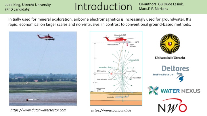
Introduction Co-authors: Gu Oude Essink, Marc.F. P. Bierkens Jude King, Utrecht University (PhD candidate) Initially used for mineral exploration, airborne electromagnetics is increasingly used for groundwater. It s rapid, economical on larger scales and non-intrusive, in contrast to conventional ground-based methods. https://www.dutchwatersector.com https://www.bgr.bund.de
Introduction Step 1: Collect Data Step 2: Inversion Conductivity (S/m) Step 3: Transform to salinity using lithological data Chloride g/l
Background Recent research has highlighted the relative sources of error for each of the three steps (see King et al., 2020). This research investigates a method to improve results. Airborne electromagnetic surveys exploit the electrical conductivity of groundwater, can we exploit another physical property to improve results? Jointly using 2 properties should be possible. ? What about density? Density https://www.youtube.com/watch?v=OMoMDsI62pY
Reducing Error Background Variable-Density Ground-Water Flow and Transport tools can simulate movement of groundwater based on density differences (fresh/saline). An aquifer that has not been changed for a long time should be in/close to equilibrium; only low velocity groundwater movements are expected. Rapid changes No/slow changes Source: Van Engelen et al., (2018) http://www.callumatkinsononline.com/animating-velocity-field-python-ffmpeg/
Background Using the idea that no rapid changes groundwater salinity should be expected, these can be used to highlight error in the resulting fresh-saline groundwater distribution. What causes these inaccuracies and how can this information be exploited? Is it: a. Inversion procedure? b. Noise from AEM acquisition? c. Groundwater model parameters? Unexpected (inaccuracies in salinity field) Fresh-water volume Set up synthetic model to investigate, then apply to real data. Previous article quantified relative error of inverse model/lithology. Expected Time (e.g. 30 years)
Reducing Error Method Summarised in 5 steps: 1. Run available groundwater model until a state of equilibrium is reached with the model boundaries and stress terms using SEAWAT code. This is now treated as a synthetic model; 2. Simulate airborne survey using standard geophysical forward modelling techniques, resulting in set of observations; 3. Invert geophysical observations and start with initial groundwater model parameters; 4. Run groundwater model in small time-steps for ~30 years; 5. Implement (downhill-simplex) optimization algorithm that penalizes rapid changes in salinity by iteratively changing groundwater model/inversion parameters.
Reducing Error Data Model/data used to construct the synthetic model: SEAWAT model from Zeeuws Vlaanderen (10 x 10km), 25m resolution, made using: Lithoclasses (and K values) from available 3D lithological model. 100m resolution, 50m depth. (Stafleu et al., 2011); Salinity data from available 3D chloride model. 50m resolution, up to ~100m depth. (Delsman et al., 2018); Available airborne data measurement locations from previous survey (Delsman et al., 2018). Initial results are promising and quantitative results will be available soon.
Thank you for looking! Comments, questions or suggestions are welcome. Delsman, J., Van Baaren, E. S., Siemon, B., Dabekaussen, W., Karaoulis, M. C., Pauw, P., et al. (2018). Large scale, probabilistic salinity mapping using airborne electromagnetics for groundwater management in Zeeland, the Netherlands. Environmental Research Letters. https://doi.org/10.1088/1748-9326/aad19e Stafleu, J., Maljers, D., Gunnink, J. L., & Busschers, F. S. (2011). 3D modelling of the shallow subsurface of Zeeland, the Netherlands, Netherlands. Journal of Geosciences, 16(1), 5647. https://doi.org/10.5242/iamg.2011.0076 King J, Oude Essink G, Karaolis M, Siemon B, Bierkens MFP (2018) Quantifying geophysical inversion uncertainty using airborne frequency domain electromagnetic data: applied at the province of Zeeland, The Netherlands. Water Resour Res 54:8420 8441. https://doi.org/10.1029/2018WR023165 Auken, E., & Christiansen, A. V. (2004). Layered and laterally constrained 2D inversion of resistivity data. Geophysics, 69(3), 752 761. https://doi.org/10.1190/1.1759461