Experimental Methods in Nuclear, Particle, and Astro Physics Overview

Physics 736: Experimental Methods in Nuclear, Particle, and Astro Physics Prof. Vandenbroucke, April 20, 2015

Announcements Problem Set 9 (last one!) due Friday 5pm Written document for report (extended outline + figures) due next Thu (Apr 30) Office hours Wed 3:45-4:45 (Chamberlin 4114) Read Barlow 7.2-8.1 for Wed (Apr 22) Read Barlow 8.2-8.4 for Mon (Apr 27)

Final presentation schedule May 13 Sida Jiande Kenneth Nick Matt Tyler Shaun May 4 Kevin M Richard Kevin G Andrew May 6 Robert Erin Sam Zach Each presentation will be 13 min + 3 min for questions For group projects, each person should give a presentation

Dead time Typically a particle detector and/or its readout electronics is dead (cannot detect another event) for some time after each event Nonparalyzable system: events that occur during the dead time do not extend the dead time Paralyzable system: events that occur during the dead time extend the dead time At high rate (time between events approaching the dead time), dead time event loss can be large and must be corrected for to infer the true rate from the measured rate Actual behavior of a system sometimes falls between these two extremes

Dead time correction in a non-paralyzable detector n = true interaction rate m = recorded rate = dead time Counting time is long: n and m are average rates Fraction of all time that detector is dead? m Rate of events lost to dead time? nm Another expression for rate of events lost to dead time? n-m So n-m = nm :

Dead time correction in a paralyzable detector Start with same definitions as non-paralyzable case An event is detected only when the time since the past (true) event occurrence is greater than What fraction of all (true) events is this? If Poisson distributed, the time T between events is exponentially distributed: So what is the probability that a given interval is greater than (this is equal to the probability that it will be detected rather than lost)? So what is the rate of events detected?

Correcting for dead time Measured rate (m) True rate (n) For both cases, in the limit of n <<1 we get the same first order correction:

Parameter estimation and curve fitting Given a set of data points and an analytical model that determines a curve, how do we determine the curve that best fits the data? Curve fitting is equivalent to applying an estimator to the data set to determine each parameter of the curve

Least squares estimation We now know how to quantitatively assess the performance of estimators (by quantifying consistency, bias, and efficiency) Is there a general prescription for how to derive a good estimator for a given problem? One powerful prescription is least squares estimation Can be used to derive an analytical form for the estimators (in terms of the data points) in the case that the functional form is a linear function of the parameters to be estimated (not necessarily a linear function of the data points) Can also be used in general, even for nonlinear functions, using numerical minimization The quantity to be minimized (with respect to a, the vector of parameters) is

Least squares fit to a straight line: summary A common special case: given data points (xi,yi) in which xi have no uncertainty and all data points yi have the same uncertainty The least squares best fit line (y=mx+c) can be determined directly from the data points with an analytical calculation: The covariance term can be avoided with an initial change of variables (by subtracting the sample mean of xi from all xi)

Generalizations of least squares estimation/fitting Uncertainty on measured dependent variable y can be constant ( ) or can vary from point to point ( i) For data point dependent errors ( i) the derivation is similar but weighted sample means etc. are used (weight is 1/ i2) y can be a histogram (with Gaussian or Poisson errors) Dependent variable y can be a function of multiple independent variables (x, z, ) e.g. fitting a plane Dependent variable can be described by a function that is linear in the parameters (analytical solution exists) or nonlinear (numerical minimization can be used) There can be uncertainty on both x and y (e.g. track fitting) Analytical solution exists if x and y are each constant across all data points Otherwise numerical solutions can be used Least squares can even be used to fit a curve that is not defined by an analytical function but is defined by a tabulation of values (a template): analytical solution can be derived if parameters are linear coefficients of the templates

Examples Can an analytical solution be found for the least squares estimators of the parameters ai in What about

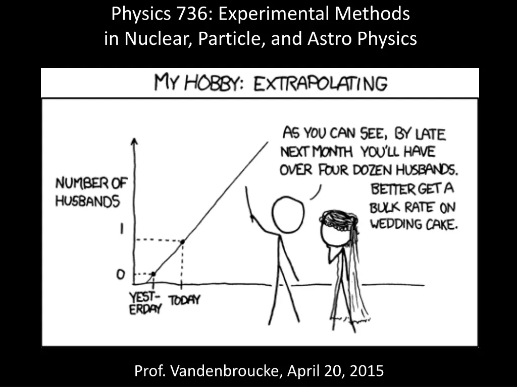
Extrapolation and interpolation Once we have a linear (or any other) fit to a model, we can use it for both interpolation and extrapolation This makes the assumption that the model is accurate in the region we are applying it, where we have not tested it (sometimes a false assumption) We can extrapolate/interpolate linearly with Under the assumption that the model holds at X, can we determine the uncertainty on our extrapolated/interpolated value Y at X? Yes: