Experimental Methods in Nuclear, Particle, and Astro Physics

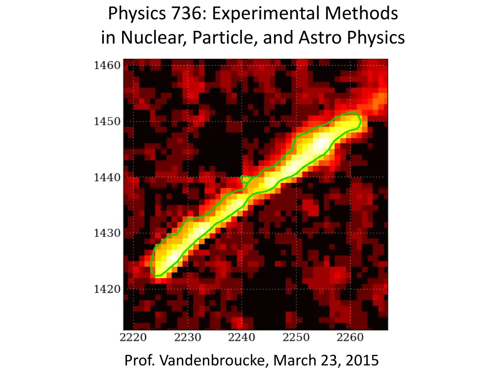
Physics 736: Experimental Methods in Nuclear, Particle, and Astro Physics Prof. Vandenbroucke, March 23, 2015

Announcements Problem Set 7 due Thursday 5pm Read Barlow 3.1-3.3 for Wed (Mar 25) Spring Break next week Read Barlow 3.4-4.2 for Mon (Apr 6) Project proposals due Mon Apr 6 5pm See details in project handout (will post on learn@uw) Send me email 1-2 paragraphs is fine If working in group, name group members Colloquium Friday: Andrea Pocar (U Mass Amherst): The present and future of solar neutrinos with Borexino, 3:30

Monte Carlo integration Number of points Approximation of 3000 3.167 30,000 3.144

Monte Carlo simulations Named after the casino destination in Monaco General method of repeated random sampling to calculate numerical results Useful for numerical integration of curves Useful for brute force simulation of particle interactions Include particle rate/flux/spectrum and interaction cross sections Some standard packages (GEANT, CORSIKA, FLUKA, ) exist Each experiment typically has one or more Monte Carlo packages for simulating the response of the detector to various signals and background (can be based on a standard such as GEANT) Two useful skills Running the fully detailed MC for a particular experiment Writing simple ( toy ) Monte Carlo simulations to answer questions about scaling and statistics quickly

Descriptive statistics Given a set of data, the first goal is to describe them quantitatively First step before answering whether the data fit a particular theory/hypothesis or fitting a parameterized model to the data (to test the model and/or measure the parameters) Simple metrics are useful: mean, mode, median (all types of average ) Standard deviation, skew, kurtosis Variance, covariance

Mean Arithmetic mean (or simply mean ) Geometric mean (e.g. for rates of growth) Harmonic mean:

Mean, mode, median Example: two different distributions (solid, hatched) with same median Mode and median are less affected by outliers than mean Mode: most probable value Median: useful when you care about the order more than the absolute value (e.g. median income)

Probability distributions For discrete random variables: probability distribution (aka probability mass function) = set of probabilities pi Normalization condition: sum of pi= 1 Units of pi: unitless For continuous random variables: probability distribution function (aka probability density function) f(x) is the probability that a random variable X lies in the interval (x, x+dx) Normalization condition: integral of f(x) = 1 Units of f(x): x-1 Expected value: the mean of a random variable (or a function of a random variable) given a probability distribution: denoted E[X] or E[f(X)]

Standard deviation Standard deviation: Sample variance: Sample standard deviation: Variance = square of standard deviation Distinction between intrinsic true variance of parent population vs. sample variance which can be used to estimate parent population variance Sample standard deviation is useful for characterizing the spread/dispersion of a set of numbers: does not imply that the distribution is Gaussian can be used to measure the width of the distribution of any set of numbers drawn from any distribution Note: RMS is often used as a shorthand for standard deviation (e.g. by ROOT), but they are only equal if the mean is subtracted Standard deviation is equal to the RMS deviation, not simply the RMS of the distribution

Useful method of calculating standard deviation

Moments and central moments nth (raw) moment = expectation value of random variable to the nth power nth central moment: mean is subtracted first Examples: zeroth moment = zeroth central moment = 1 First raw moment = mean (expected value) First central moment = 0 Second central moment = variance Standardized central moment: divide by n nth central moment ( n):

Skewness (aka skew) Skewness is the third standardized moment Useful for quantifying how symmetric a distribution is about the mean

Covariance Given two jointly distributed random variables (X,Y) Jointly distributed means the data come in pairs, not necessarily that they are correlated or dependent on one another Cov(X,Y) = E[(X-E[X])(Y-E[Y])] = E[XY] E[X]E[Y] Units of covariance are [units of X]*[units of Y] If X and Y are independent, their covariance is zero If X=Y, covariance = variance For two or more variables, covariances can be assembled in a matrix Covariance matrix is symmetric (diagonal entries are variances)

(Pearson) correlation coefficient Divide the covariance by the variances to determine a dimensionless measure of the degree of correlation of two random variables +1: perfectly positively correlated (slope does not matter) -1: perfectly negatively correlated (anti-correlated; slope does not matter) 0: not linearly correlated (can be correlated in nonlinear ways: see bottom row)