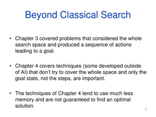
Exploring Blind and Depth-First Search Algorithms in AI
"Discover the Blind Breadth First Search and Depth First Search algorithms, commonly used by researchers in AI. Learn how these algorithms define problems, states, and rules through examples and solutions involving a farmer crossing a river with a wolf, goose, and bundle of rice."

Download Presentation

Please find below an Image/Link to download the presentation.
The content on the website is provided AS IS for your information and personal use only. It may not be sold, licensed, or shared on other websites without obtaining consent from the author. If you encounter any issues during the download, it is possible that the publisher has removed the file from their server.
You are allowed to download the files provided on this website for personal or commercial use, subject to the condition that they are used lawfully. All files are the property of their respective owners.
The content on the website is provided AS IS for your information and personal use only. It may not be sold, licensed, or shared on other websites without obtaining consent from the author.
E N D
Presentation Transcript
Algoritma Pencarian Blind Breadth First Search Depth First Search
Deskripsi Merupakan algoritma untuk mencari kemungkinan penyelesaian Sering dijumpai oleh peneliti di bidang AI
Mendefinisikan permasalahan Mendefinisikan suatu state (ruang keadaan) Menerapkan satu atau lebih state awal Menetapkan satu atau lebih state tujuan Menetapkan rules (kumpulan aturan)
A unifying view (Newell and Simon) Ruang masalah terdiri dari: state space adalah himpunan state yang mungkin dari suatu permasalahan Himpunan operators digunakan untuk berpindah dari satu state ke state yang lain. Ruang masalah dapat digambarkan dengan graph, himpunan state dinyatakan dengan node dan link (arcs) menyatakan operator.
Contoh 1 Seorang petani ingin memindah dirinya sendiri, seekor serigala, seekor angsa gemuk, dan seikat padi yang berisi menyeberangi sungai. Sayangnya, perahunya sangat terbatas; dia hanya dapat membawa satu objek dalam satu penyeberangan. Dan lagi, dia tidak bisa meninggalkan serigala dan angsa dalam satu tempat, karena serigala akan memangsa angsa. Demikian pula dia tidak bisa meninggalkan angsa dengan padi dalam satu tempat.
State (ruang keadaan) State (Serigala, Angsa, Padi, Petani) Daerah asal ketika hanya ada serigala dan padi, dapat direpresentasikan dengan state (1, 0, 1, 0), sedangkan daerah tujuan adalah (0, 1, 0, 1)
State awal dan tujuan State awal Daerah asal (1, 1, 1, 1) Darah tujuan (0, 0, 0, 0) State tujuan Daerah asal (0, 0, 0, 0) Darah tujuan (1, 1, 1, 1)
Rules Aturan ke 1 Rule Angsa menyeberang bersama petani 2 Padi menyeberang bersama petani 3 Serigala menyeberang bersama petani 4 Angsa kembali bersama petani 5 Padi kembali bersama petani 6 Serigala kembali bersama petani 7 Petani kembali
Contoh solusi Daerah asal (S, A, Pd, Pt) (1, 1, 1, 1) (1, 0, 1, 0) (1, 0, 1, 1) (0, 0, 1, 0) (0, 1, 1, 1) (0, 1, 0, 0) (0, 1, 0, 1) (0, 0, 0, 0) Daerah tujuan (S, A, Pd, Pt) (0, 0, 0, 0) (0, 1, 0, 1) (0, 1, 0, 0) (1, 1, 0, 1) (1, 0, 0, 0) (1, 0, 1, 1) (1, 0, 1, 0) (1, 1, 1, 1) Rule yang dipakai 1 7 3 4 2 7 1 solusi
F W D C W D C D C W C W D F F W F D F C F W C F W D C D W C C W F D F W D F D C F C F W C F D C F W F W D F W C W D D W D C C D D C C D W D D W F W F W D F W C F C F W C F D C F D F W D F D C W C C W Last time we saw D F W C F W D C Search Tree for Farmer, Wolf, Duck, Corn Repeated State Illegal State Goal State
Contoh 2 Eight Puzzle 1 4 3 1 4 3 7 6 2 7 6 5 8 5 8 2
State space of the 8-puzzle generated by move blank operations
The 8-puzzle problem as state space search State Operator Initial state (state awal) telah ditentukan Goal state (state akhir) telah ditentukan : posisi board yang legal : up, left, down, right : posisi board yang : posisi board yang Catatan : Yang ditekankan disini bukan solusi dari 8-puzzle, tapi lintasan/path dari state awal ke state tujuan.
Contoh 3 Traveling Salesperson Problem
Traveling salesperson problem as state space search The salesperson has n cities to visit and must then return home. Find the shortest path to travel. state space: operators: initial state: goal state:
Search of the traveling salesperson problem. (arc label = cost from root)
Nearest neighbor path Nearest neighbor path = AEDBCA (550) Minimal cost path = ABCDEA (375)
Search Breadth-First Search DEPTH 0 (d=0) DEPTH 1 (d=1) DEPTH 2 (d=2)
Search strategies - BFS BreadthFirstSearch(state space =<S,P,I,G,W>) Open {I} Closed while Open do x DeQueue(Open) ifGoal(x, ) then return x Insert(x,Closed) for y Child(x , ) do if y Closed and y Open then EnQueue(y,Open) returnfail Open is implemented as queue (FIFO); Closed can be an arbitrary data structure for sets
Breath-first search S A D B D A E C 11 E E B B F D 14 F B F C 17 E A 15 C 15 G 13 G 19 C 19 G 17 F G 25
Search strategies - DFS DepthFirstSearch(state space =<S,P,I,G,W>) Open {I} Closed while Open do x Pop(Open) ifGoal(x, ) then return x Insert(x,Closed) for y Child(x , ) do if y Closed and y Open then Push(y,Open) returnfail Open is implemented as stack (LIFO); Closed can be an arbitrary data structure for sets
Depth-first search S A D B D A E C 11 E E B B F D 14 F B F C 17 E A 15 C 15 G 13 G 19 C 19 G 17 F G 25
BFS, label = order state was removed from OPEN
DFS with a depth bound of 5, label = order state was removed from OPEN
Blind search BFS dan DFS disebut Blind search dalam arti bahwa metode ini tidak memiliki pengetahuan tentang masalah sama sekali selain ruang permasalahan Metode BFS dan DFS disebut juga brute-force search, uninformed search, atau weak method Dengan metode ini tidak dapat berharap terlalu banyak, tapi metode ini memberikan: - Worst-case scenarios - dasar dari algoritma berikutnya
Search strategies A search strategy is defined by picking the order of node expansion Strategies are evaluated along the following dimensions: completeness: does it always find a solution if one exists? time complexity: number of nodes generated space complexity: maximum number of nodes in memory optimality: does it always find a least-cost solution? Time and space complexity are measured in terms of b: maximum branching factor of the search tree d is the depth of the solution m is the maximum depth of the tree 14 Jan 2004 CS 3243 - Blind Search 44
Properties of BFS dan DFS Completeness: (Does it always find a solution?) Time complexity: (How long does it take?) Space complexity: (How much memory does it take?) Optimality: (Does it always insure the best )
Properties of breadth-first search Completeness: Yes, if b is finite Time complexity: O(b d), i.e., exponential in d (Rem: b is no. of branches) Space complexity: O(b d), keeps every node in memory Optimality: where b is the branching factor, d is the depth of the solution Yes, if cost = 1 per step; not optimal in general
Kelebihan BFS Tidak akan menemui jalan buntu Jika ada satu solusi, maka BFS akan menemukannya. Dan jika ada lebih dari satu solusi, maka solusi minimum akan ditemukan.
Kelemahan BFS Membutuhkan memori yang cukup banyak, karena menyimpan semua node dalam satu pohon. Membutuhkan waktu yang cukup lama, karena akan menguji n level untuk mendapatkan solusi pada level ke-(n+1)
Properties of depth-first search Completeness: Time complexity: terrible if m is much larger than d but if solutions are dense, may be much faster than breadth-first Space complexity: O(bm) Optimality: No No, fails in infinite state-space O(b m) where b is the branching factor, m is the maximum depth of the tree
Kelebihan DFS Membutuhkan memori yang relatif kecil, karena hanya node-node pada lintasan yang aktif saja yang disimpan. Secara kebetulan, metode DFS akan menemukan solusi tanpa harus menguji lebih banyak lagi dalam ruang keadaan.


")

")


")


")


")