Exponents, Logarithms, and Their Applications
Examine the fundamental concepts of exponents and logarithms in nature and various disciplines. Explore how exponential expressions describe processes like diffusion, chemical reactions, and pharmacokinetics. Learn about the significance of logarithmic scales in different fields, such as acoustics, photography, and earthquake measurement, providing insights into complex phenomena.

Uploaded on Apr 04, 2025 | 2 Views
Download Presentation

Please find below an Image/Link to download the presentation.
The content on the website is provided AS IS for your information and personal use only. It may not be sold, licensed, or shared on other websites without obtaining consent from the author.If you encounter any issues during the download, it is possible that the publisher has removed the file from their server.
You are allowed to download the files provided on this website for personal or commercial use, subject to the condition that they are used lawfully. All files are the property of their respective owners.
The content on the website is provided AS IS for your information and personal use only. It may not be sold, licensed, or shared on other websites without obtaining consent from the author.
E N D
Presentation Transcript
Clinical Pharmacokinetic Equations and Calculations Dr. Haider Raheem Mohammad
Introduction The value of Pi ( ) is the ratio of the circumference of a circle to its diameter and is approximately equal to 3.14159 (3.14159265 ). In a circle, if you divide the circumference (is the total distance around the circle) by the diameter, you will get exactly the same number. Whether the circle is big or small, the value of pi remains the same.
Exponents and Logarithms For many processes in nature, the rate of removal or modification of a species is proportional to, and driven by, the amount of that species present at a given time. This is true for the kinetics of diffusion, for chemical reactions, for radioactive decay, and for the kinetics of the ADME processes of pharmaceuticals. Systems of this type are naturally described by exponential expressions.
Exponents and Logarithms Exponential processes in nature have the number e (equaling 2.7183. . . ) for the base. For example, e1= 2.7183 The inverse operation, ln, will return the original exponent: ln(e1) = ln(2.7183 ) = 1.
Exponents and Logarithms Since we humans have 10 digits and are used to counting in the decimal system, we often use the base 10, for which the inverse logarithmic operation is called log. For example, 102= 100, and log(102) = log(100) = 2. The interconversion between expressions containing logs and expressions containing lns by use of the number 2.303, which is simply ln(10).
Exponents and Logarithms The widely quoted Richter scale is one example of a widely used base 10 logarithmic measure. It was devised by Charles Richter in 1935 to compare earthquake magnitudes. As you know from news reports, on the Richter scale, an earthquake of, say, magnitude 5 is ten times a magnitude 4, and so on. A major earthquake has magnitude 7, while a magnitude 8 or larger is called a Great Quake.AGreat Quake can destroy an entire community.
Exponents and Logarithms Other logarithmic scales include the decibel in acoustics, the octave in music, f-stops in photographic exposure, and entropy in thermodynamics. The pH scale chemists use to measure acidity and the stellar magnitude scale used by astronomers to measure the star brightness are also examples of logarithmic scales.
Exponents and Logarithms Most calculators have two logarithmic keys: logx and lnx. The log x has a base 10 (log10x) and ln x has a base e (logex). Base 10 logarithms are called common logarithms, while base e logarithms are called natural logarithms. Note that the base numerals 10 and e are identified by the symbolic spelling log and ln, respectively.
Exponents and Logarithms 100= 1 101= 10 102= 100 103= 1000 104= 10000 105= 100000 106= 1000000 log(1) = 0 log(10) = 1 log(100) = 2 log(1000) = 3 log(10000) = 4 log(100000) = 5 log(1000000) = 6
Exponents and Logarithms 100= 1 10-1= 0.1 10-2= 0.01 10-3= 0.001 10-4= 0.0001 10-5= 0.00001 10-6= 0.000001 log(1) = 0 log(0.1) = -1 log(0.01) = -2 log(0.001) = -3 log(0.0001) = -4 log(0.00001) = -5 log(0.000001) = -6
Hierarchy of arithmetic operations (in order from high to low)
One-Compartment Model Equations for Linear Pharmacokinetics In many cases, the drug distributes from the blood into the tissues quickly, and a pseudoequilibrium of drug movement between blood and tissues is established rapidly. When this occurs, a one-compartment model can be used to describe the serum concentrations of a drug. In some clinical situations, it is possible to use a one-compartment model to compute doses for a drug even if drug distribution takes time to complete. In this case, drug serum concentrations are not obtained in a patient until after the distribution phase is over.
One-Compartment Model Equations for Linear Pharmacokinetics The simplest model is the one-compartment model which depicts the body as one large container where drug distribution between blood and tissues occurs instantaneously. Drug is introduced into the compartment by infusion (k0), absorption (ka), or IV bolus; distributes immediately into a volume of distribution (V); and is removed from the body via metabolism and elimination via the elimination rate constant (ke). The simplest multicompartment model is a two-compartment model which represents the body as a central compartment into which drug is administered and a peripheral compartment into which drug distributes. Rate constants (k12, k21) represent the transfer between compartments and elimination from the body (k10).
Intravenous Bolus Equation When a drug is given as an intravenous bolus and the drug distributes from the blood into the tissues quickly, the serum concentrations often decline in a straight line when plotted on semilogarithmic axes. In this case, a one-compartment model intravenous bolus equation can be used: C = (D/V) e ket where t is the time after the intravenous bolus was given (t = 0 at the time the dose was administered), C is the concentration at time = t, V is the volume of distribution, and keis the elimination rate constant.
Intravenous Bolus Equation The solid line shows the serum concentration/time graph for a drug that follows one-compartment model pharmacokinetics after intravenous bolus administration. Drug distribution occurs instantaneously, and serum concentrations decline in a straight line on semilogarithmic axes. The dashed line represents the serum concentration/time plot for a drug pharmacokinetics after an intravenous bolus is given. Immediately after the dose is given, serum concentrations decline rapidly. This portion of the curve is known as the distribution phase. that follows two-compartment model
Intravenous Bolus Equation Most drugs given intravenously cannot be given as an actual intravenous bolus because of side effects related to rapid injection. A short infusion of 5 30 minutes can avoid these types of adverse effects, and if the intravenous infusion time is very short compared to the half-life of the drug so that a large amount of drug is not eliminated during the infusion time, intravenous bolus equations can still be used.
Intravenous Bolus Equation For example, a patient is given a theophylline loading dose of 400 mg intravenously over 20 minutes. theophylline during previous hospitalizations, it is known that the volume of distribution is 30 L, the elimination rate constant equals 0.115 h 1, and the half-life (t1/2) is 6 hours (t1/2= 0.693/ke= 0.693/0.115 h 1= 6 h). To compute the expected theophylline concentration 4 hours after the dose was given, a one-compartment model intravenous bolus equation can be used: C = (D/V) e ket = (400 mg/30 L) e (0.115 h 1)(4 h)= 8.4 mg/L. Because the patient received
Intravenous Bolus Equation If drug distribution is not rapid, it is still possible to use a one compartment model intravenous bolus equation if the duration of the distribution phase and infusion time is small compared to the half-life of the drug and only a small amount of drug is eliminated during the infusion and distribution phases. For instance, vancomycin must be infused slowly over 1 hour in order to avoid hypotension and red flushing around the head and neck areas. Additionally, vancomycin distributes slowly to tissues with a distribution phase. Because the half-life of vancomycin in patients with normal renal function is approximately 8 hours, a one compartment model intravenous bolus equation can be used to compute concentrations in the postinfusion, postdistribution phase without a large amount of error. 1/2 1 hour
Intravenous Bolus Equation As an example of this approach, a patient is given an intravenous dose of vancomycin 1000 mg. Since the patient has received this drug before, it is known that the volume of distribution equals 50 L, the elimination rate constant is 0.077 h 1, and the half-life equals 9 h (t1/2= 0.693/ke= 0.693/0.077 h 1= 9 h). To calculate the expected vancomycin concentration 12 hours after the dose was given, a one compartment model intravenous bolus equation can be used: C = (D/V) e ket = (1000 mg / 50 L) e (0.077 h 1)(12 h)= 7.9 mg/L.
Intravenous Bolus Equation Pharmacokinetic parameters for patients can also be computed for use in the equations. If two or more serum concentrations are obtained after an intravenous bolus dose, the elimination rate constant, half-life and volume of distribution can be calculated. For example, a patient was given an intravenous loading dose of phenobarbital 600 mg over a period of about an hour. One day and four days after the dose was administered concentrations were 12.6 mg/L and 7.5 mg/L, respectively. phenobarbital serum
Intravenous Bolus Equation Phenobarbital concentrations are plotted on semilogarithmic axes, and a straight line is drawn connecting the concentrations. Half-life (t1/2) is determined by measuring the time needed for serum concentrations to decline by1/2(i.e., from 12.6 mg/L to 6.3 mg/L), and is converted to the elimination rate constant (ke= 0.693/t1/2 = 0.693/4d = 0.173d 1). The concentration/time line can be extrapolated to the concentration axis to derive the concentration at time zero (C0= 15 mg/L) and used to compute the volume of distribution (V = D/C0).
Intravenous Bolus Equation By plotting the serum concentration/time data on semilogarithmic axes, the time it takes for serum concentrations to decrease by one-half can be determined and is equal to 4 days. The elimination rate constant can be computed using the following relationship: ke= 0.693/t1/2= 0.693/4 d = 0.173 d 1. The concentration/time line can be extrapolated to the y-axis where time = 0. Since this was the first dose of phenobarbital and the predose concentration was zero, the extrapolated concentration at time = 0 (C0= 15 mg/L in this case) can be used to calculate the volume of distribution.
Intravenous Bolus Equation For a one-compartment model, the body can be thought of as a beaker containing fluid. If 600 mg of phenobarbital is added to a beaker of unknown volume and the resulting concentration is 15 mg/L, the volume can be computed by taking the quotient of the amount placed into the beaker and the concentration: V = D/C0= 600 mg/(15 mg/L) = 40 L.
Intravenous Bolus Equation Alternatively, these parameters could be obtained by calculation without plotting the concentrations. The elimination rate constant can be computed using the following equation: ke= (ln C1 ln C2)/(t1 t2) where t1and C1are the first time/concentration pair and t2and C2are the second time/concentration pair; ke= [ln (12.6 mg/L) ln (7.5 mg/L)]/(1 d 4 d) = 0.173 d 1. The elimination rate constant can be converted into the half-life using the following equation: t1/2= 0.693/ke= 0.693/0.173 d 1= 4 d.
Intravenous Bolus Equation The volume of distribution can be calculated by dividing the dose by the serum concentration at time = 0. The serum concentration at time = zero (C0) can be computed using a variation of the intravenous bolus equation: C0= C/e ket where t and C are a time/concentration pair that occur after the intravenous bolus dose. Either phenobarbital concentration can be used to compute C0. In this case, the time/concentration pair on day 1 will be used (time = 1 d, concentration = 12.6 mg/L): C0= C/e ket= (12.6 mg / L) / e (0.173 d 1)(1 d)= 15.0 mg/L. The volume of distribution (V) is then computed: V = D/ C0= 600 mg / (15 mg/L) = 40 L.
Continuous and Intermittent Intravenous Infusion Equations Some drugs are administered using a continuous intravenous infusion, and if the infusion is discontinued the serum concentration/time profile decreases in a straight line when graphed on a semilogarithmic axes. If a drug is given as a continuous intravenous infusion, serum concentrations increase until a steady-state concentration (Css) is achieved in 5 7 half-lives. The steady-state concentration is determined by the quotient of the infusion rate (k0) and drug clearance (Cl): Css = k0/Cl. When the infusion is discontinued, serum concentrations decline in a straight line if the graph is plotted on semilogarithmic axes. When using log10graph paper, the elimination rate constant (ke) can be computed using the following formula: slope = ke/2.303.
Continuous and Intermittent Intravenous Infusion Equations In this case, a one compartment model intravenous infusion equation can be used to compute concentrations (C) while the infusion is running: C = (k0/Cl)(1 e ket) = [k0/(keV)](1 e ket) where k0is the drug infusion rate (in amount per unit time, such as mg/h or g/min), Cl is the drug clearance (since Cl = keV, this substitution was made in the second version of the equation), keis the elimination rate constant, and t is the time that the infusion has been running. If the infusion is allowed to continue until steady state is achieved, the steady-state concentration (Css) can be calculated easily: Css = k0/ Cl = k0/ (keV)
Continuous and Intermittent Intravenous Infusion Equations If the infusion is stopped, postinfusion serum concentrations (Cpostinfusion) can be computed by calculating the concentration when the infusion ended (Cend) using the appropriate equation in the preceding paragraph, and the following equation: Cpostinfusion= Cende ketpostinfusion where keis the elimination rate constant and tpostinfusionis the postinfusion time (tpostinfusion= 0 at end of infusion and increases from that point).
Continuous and Intermittent Intravenous Infusion Equations Even if serum concentrations exhibit a distribution phase after the drug infusion has ended, it is still possible to use one compartment model intravenous infusion equations for the drug without a large amount of error. For example, gentamicin, tobramycin, and amikacin are usually infused over one-half hour. When administered this way, these aminoglycoside antibiotics have distribution phases that last about one-half hour. Using this strategy, aminoglycoside serum concentrations are obtained no sooner than one-half hour after a 30-minute infusion in order to avoid the distribution phase. If aminoglycosides are infused over 1 hour, the distribution phase is very short and serum concentrations can be obtained immediately.
Continuous and Intermittent Intravenous Infusion Equations For example, a patient is given an intravenous infusion of gentamicin 100 mg over 60 minutes. Because the patient received gentamicin before, it is known that the volume of distribution is 20 L, the elimination rate constant equals 0.231 h 1, and the half-life equals 3 h (t1/2= 0.693/ke= 0.693/0.231 h 1 = 3 h). To compute the gentamicin concentration at the end of infusion, a one compartment model intravenous infusion equation can be employed: C = [k0/(keV)](1 e ket) = [(100 mg/1 h)/(0.231 h 1 20 L)](1 e (0.231 h 1)(1 h)) = 4.5 mg/L.
Continuous and Intermittent Intravenous Infusion Equations If the infusion did not run until steady state was achieved, it is still possible to compute pharmacokinetic parameters from postinfusion concentrations. In the following example, a patient was given a single 120-mg dose of tobramycin as a 60-minute infusion, and concentrations at the end of infusion (6.2 mg/L) and 4 hours after the infusion ended (1.6 mg/L) were obtained. By plotting the serum concentration/time semilogarithmic axes, the half-life can be determined by measuring the time it takes for serum concentrations to decline by one-half, and equals 2 hours in this case. information on
Continuous and Intermittent Intravenous Infusion Equations Tobramycin concentrations are plotted on semilogarithmic axes, and a straight line is drawn connecting the concentrations. Half-life (t1/2) is determined by measuring the time needed for serum concentrations to decline by1/2(i.e., from 6.2 mg/L to 3.1 mg/L), and is converted to the elimination rate constant (ke= 0.693/ t1/2= 0.693/2 h = 0.347 h 1).
Continuous and Intermittent Intravenous Infusion Equations The elimination rate constant (ke) can be calculated using the following formula: ke= 0.693/t1/2= 0.693/2 h = 0.347 h 1. Alternatively, the elimination rate constant can be calculated without plotting the concentrations using the following equation: ke= (ln C1 ln C2)/(t1 t2) where t1and C1are the first time/concentration pair and t2and C2are the second time/concentration pair; ke= [ln (6.2 mg/L) ln (1.6 mg/L)] / (1 h 5 h) = 0.339 h 1(note the slight difference in keis due to rounding errors). The elimination rate constant can be converted into the half-life using the following equation: t1/2= 0.693/ ke= 0.693/0.339 h 1= 2 h.
Continuous and Intermittent Intravenous Infusion Equations The volume of distribution (V) can be computed using the following equation: ??(1 e ket ) ??[???? (Cpredosee ket ) where k0is the infusion rate, keis the elimination rate constant, t = infusion time, Cmaxis the maximum concentration at the end of infusion, and Cpredoseis the predose concentration. In this example, the volume of distribution is: V = (120 mg/1 h) (1 e (0.339h 1)(1h)) 0.339 h 1[(6.2 mg/L) (0 mg/L e (0.339h 1)(1h))= 16.4 L V =
Extravascular Equation When a drug is administered extravascularly (e.g., orally, intramuscularly, subcutaneously, transdermally, etc.), absorption into the systemic vascular system must take Place. The absorption rate constant (ka) controls how quickly the drug enters the body. A large absorption rate constant allows drug to enter the body quickly while a small elimination rate constant permits drug to enter the body more slowly. The solid line shows the concentration/time curve on semilogarithmic axes for an absorption rate constant equal to 2 h 1. The dashed and dotted lines depict serum concentration/time plots for absorption rate constants of 0.5 h 1and 0.2 h 1, respectively.
Extravascular Equation If serum concentrations decrease in a straight line when plotted on semilogarithmic axes after drug absorption is complete, a one compartment model extravascular equation can be used to describe the serum concentration/time curve: C = {(FkaD) / [V(ka ke)]}(e ket e kat) where t is the time after the extravascular dose was given (t = 0 at the time the dose was administered), C is the concentration at time = t, F is the bioavailability fraction, kais the absorption rate constant, D is the dose, V is the volume of distribution, and keis the elimination rate constant.
Extravascular Equation An example of the use of this equation would be a patient that is administered 500 mg of oral procainamide as a capsule. It is known from prior clinic visits that the patient has a half-life equal to 4 hours, an elimination rate constant of 0.173 h 1(ke= 0.693/t1/2= 0.693/4 h = 0.173 h 1), and a volume of distribution of 175 L. The capsule that is administered to the patient has an absorption rate constant equal to 2 h 1, and an oral bioavailability fraction of 0.85. The procainamide serum concentration 4 hours after a single dose would be equal to: ???? ? (?? ??)(e ket e kat) 2 h 1(500 mg) (175 L) (2h 1 0.173h 1)(e (0.173h 1)(4h) e (2h 1)(4h)) = 1.3 mg/L C = 0.85 C =
Extravascular Equation Since the absorption rate constant is also hard to measure in patients, it is also desirable to avoid drawing drug serum concentrations during the absorption phase in clinical situations. postdistribution serum concentrations are obtained for a drug that is administered extravascularly, the equation simplifies to: C = [(FD)/V] e ket where C is the concentration at any postabsorption, postdistribution time; F is the bioavailability fraction; D is the dose; V is the volume of distribution; keis the elimination rate constant; and t is any postabsorption, postdistribution time. This approach works very well when the extravascular dose is rapidly absorbed and not a sustained- or extended-release dosage form. When only postabsorption,
Extravascular Equation An example would be a patient receiving 24 mEq of lithium ion as lithium carbonate capsules. From previous clinic visits, it is known that the patient has a volume of distribution of 60 L and an elimination rate constant equal to 0.058 h 1. The bioavailability of the capsule is known to be 0.90. The serum lithium concentration 12 hours after a single dose would be: C = [(FD)/V] e ket = [(0.90 24 mEq)/60 L] e (0.058 h 1)(12 h) = 0.18 mEq/L.
Extravascular Equation If two or more postabsorption, postdistribution serum concentrations are obtained after an extravascular dose, the volume of distribution, elimination rate constant, and half-life can be computed. Valproic acid concentrations are plotted on semilogarithmic axes, and a straight line is drawn connecting the concentrations. Half-life (t1/2) is determined by measuring the time needed for serum concentrations to decline by1/2(i.e., from 51.9 mg/L to 26 mg/L), and is converted to the elimination rate constant (ke= 0.693/t1/2= 0.693/14 h = 0.0495 h 1). The concentration/ time line can be extrapolated to the concentration axis to derive the concentration at time zero (C0= 70 mg/L) and used to compute the hybrid constant volume of distribution/bioavailability fraction (V/F = D/C0).
Extravascular Equation For example, a patient is given an oral dose of valproic acid 750 mg as capsules. Six and twenty-four hours after the dose, the valproic acid serum concentrations are 51.9 mg/L and 21.3 mg/L, respectively. After graphing the serum concentration/time data on semilogarithmic axes, the time it takes for serum concentrations to decrease by one-half can be measured and equals 14 hours. The elimination rate constant is calculated using the following equation: ke = 0.693 / t1/2= 0.693/14 h = 0.0495 h 1. The concentration/time line can be extrapolated to the y-axis where time = 0. Since this was the first dose of valproic acid, the extrapolated concentration at time = 0 (C0= 70 mg/L) is used to estimate the hybrid volume of distribution/bioavailability (V/F) parameter: V/F = D/C0= 750 mg/70 L = 10.7 L. Even though the absolute volume of distribution and bioavailability cannot be computed without the administration of intravenous drug, the hybrid constant can be used in extravascular equations in place of V/F.
Extravascular Equation An alternative approach is to directly calculate the parameters without plotting the concentrations. The elimination rate constant (ke) is computed using the following relationship: ke= (ln C1 ln C2) / (t1 t2) where C1is the first concentration at time = t1, and C2is the second concentration at time = t2; ke= [ln (51.9 mg/L) ln (21.3 mg/L)] / (6 h 24 h) = 0.0495 h 1. The elimination rate constant can be translated into the half-life using the following equation: t1/2= 0.693/ke= 0.693/0.0495 h 1= 14 h.
Extravascular Equation The extrapolated serum concentration at time = zero (C0) is calculated using a variation of the intravenous bolus equation: C0= C/e ket where t and C are a time/concentration pair that occur after administration of the extravascular dose in the postabsorption and postdistribution phases. Either valproic acid concentration can be used to compute C0. In this situation, the time/concentration pair at 24 hours will be used (time = 24 hours, concentration = 21.3 mg/L): C0= C/e ket= (21.3 mg/L) / e (0.0495 h 1)(24 h)= 70 mg/L. The hybrid volume of distribution/bioavailability constant (V/F) is then computed: V/F = D/C0= 750 mg / (70 mg/L) = 10.7 L.
Multiple-Dose and Steady-State Equations In most cases, medications are administered to patients as multiple doses, and drug serum concentrations for therapeutic drug monitoring are not obtained until steady state is achieved. For these reasons, multiple dose equations that reflect steady-state conditions are usually more useful in clinical settings than single dose equations. Fortunately, it is simple to convert single dose compartment model equations to their multiple dose and steady-state counterparts. In order to change a single dose equation to the multiple dose version, it is necessary to multiply each exponential term in the equation by the multiple dosing factor: (1 e nki )/(1 e ki ) where n is the number of doses administered, kiis the rate constant found in the exponential of the single dose equation, and is the dosage interval.
Multiple-Dose and Steady-State Equations At steady state, the number of doses (n) is large, the exponential term in the numerator of the multiple dosing factor ( nki ) becomes a large negative number, and the exponent approaches zero. Therefore, the steady-state version of the multiple dosing factor becomes the following: 1/(1 e ki ) where kiis the rate constant found in the exponential of the single dose equation and is the dosage interval. Whenever the multiple dosing factor is used to change a single dose equation to the multiple dose or steady-state versions, the time variable in the equation resets to zero at the beginning of each dosage interval.
Multiple-Dose and Steady-State Equations As an example of the conversion of a single dose equation to the steady-state variant, the one compartment model intravenous bolus equation is: C = (D/V) e ket Since there is only one exponential in the equation, the multiple dosing factor at steady state is multiplied into the expression at only one place, substituting the elimination rate constant (ke) for the rate constant in the multiple dosing factor: C = (D/V) [e ket / (1 e ke )] where C is the steady-state concentration at any postdose time (t) after the dose (D) is given, V is the volume of distribution, ke is the elimination rate constant, and is the dosage interval.
Multiple-Dose and Steady-State Equations The calculations is in the computation of the volume of distribution. When a single dose of medication is given, the predose concentration is assumed to be zero. However, when multiple doses are given, the predose concentration is not usually zero, and the volume of distribution equation (V) needs to have the baseline, predose concentration (Cpredose) subtracted from the extrapolated drug concentration at time = 0 (C0) for the intravenous bolus (V = D/[C0 Cpredose], where D is dose) and extravascular (V/F = D/[C0 Cpredose], where F is the bioavailability fraction and D is dose) cases. main difference between single-dose and multiple-dose
Multiple-Dose and Steady-State Equations In the case of intermittent intravenous infusions, the volume of distribution equation already has a parameter for the predose concentration in it: ??(1 e ket ) ??[???? (Cpredosee ket ) where k0is the infusion rate, keis the elimination rate constant, t = infusion time, Cmaxis the maximum concentration at the end of infusion, and Cpredoseis the predose concentration. For each route of administration, the elimination rate constant (ke) is computed using the same equation as the single dose situation: ke= (ln C1 ln C2) / (t1 t2), where C1is the first concentration at time = t1, and C2is the second concentration at time = t2. V =