Filtered Complexes: An Increasing Sequence of Simplicial Complexes
In mathematics, a filtered complex is a sequence of simplicial complexes where each complex is a subset of the next, ordered by inclusion. Learn more about filtered complexes and their properties in this insightful article. Discover how these structures are crucial in various areas of mathematics, such as algebraic topology and combinatorics. Delve into the link between filtered complexes and other mathematical concepts to deepen your understanding of this fascinating topic.

Download Presentation

Please find below an Image/Link to download the presentation.
The content on the website is provided AS IS for your information and personal use only. It may not be sold, licensed, or shared on other websites without obtaining consent from the author.If you encounter any issues during the download, it is possible that the publisher has removed the file from their server.
You are allowed to download the files provided on this website for personal or commercial use, subject to the condition that they are used lawfully. All files are the property of their respective owners.
The content on the website is provided AS IS for your information and personal use only. It may not be sold, licensed, or shared on other websites without obtaining consent from the author.
E N D
Presentation Transcript
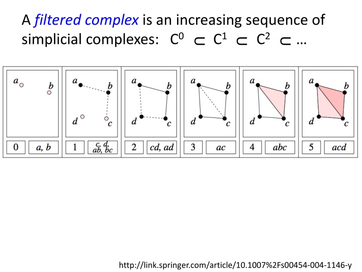
A filtered complex is an increasing sequence of simplicial complexes: C0 C1 C2 U U U http://link.springer.com/article/10.1007%2Fs00454-004-1146-y
A filtered complex is an increasing sequence of simplicial complexes: C0 C1 C2 U U U a, b is in C0 C1 C2 C5 0 0 U U U U 0 0 {a, b, c} is in C4 C5 U 2 2 http://link.springer.com/article/10.1007%2Fs00454-004-1146-y
A filtered complex is an increasing sequence of simplicial complexes: C0 C1 C2 U U U
Barcode for H0 H0 = Z0/B0 = cycles boundaries
Barcode for H1 H1 = Z1/B1 = cycles boundaries
Barcode for H2 H2 = Z2/B2 = cycles boundaries
Topological Persistence and Simplification:link.springer.com/article/10.1007/s00454-002-2885-2
Computing Persistent Homology by Afra Zomorodian, Gunnar Carlsson i, p Hk = Zk /(Bk Zk ) i i+p i U http://link.springer.com/article/10.1007%2Fs00454-004-1146-y
<z1, z2 : tz2, t3z1 + t2z2 > where z1 = ad + cd + t(bc) + t(ab), z2 = ac + t2bc + t2ab i, p i i+p i U H1 = Z1 /(B1 Z1 ) deg z1 = 2, deg z2 = 3, deg tz2 = 4, deg t3z1 + t2z2 = 5
H0 = < a, b, c, d : tc + td, tb + c, ta + tb> H1 = <z1, z2 : t z2, t3z1 + t2z2 > [ ) [ ) [ ) [ ) [ z1 = ad + cd + t(bc) + t(ab), z2 = ac + t2bc + t2ab
To install the TDA package on a PC: install.packages("TDA") To install the TDA package on a Mac: install.packages("TDA", type = "source") XX = circleUnif(30)
Barcode Persistence Diagram
Bottleneck Distance. Let Diag1and Diag2 be persistence diagrams. The bottleneck distance is the infimum over all bijections h: Diag1 Diag 2 of supi d(i; h(i)).
(Wasserstein distance). The p-th Wasserstein distance between two persistence diagrams, d1 and d2, is defined as where ranges over all bijections from d1 to d2.
> print( bottleneck(Diag1, Diag2, dimension=0) ) [1] 0.4942465 > print( wasserstein(Diag1, Diag2, p=2, dimension=0) ) [1] 5.750874 > print( bottleneck(Diag1, Diag2, dimension=1) ) [1] 0.279019 > print( wasserstein(Diag1, Diag2, p=2, dimension=1) ) [1] 0.301575


. The p-th Wasserstein")
 )")