Finding Nearest Common Ancestors in Trees - Algorithms and Methods
Explore various algorithms and techniques for efficiently finding nearest common ancestors in trees, including preprocessing time comparisons, Cartesian tree construction, discrete range maximum, reduction techniques, and NCA on perfect binary trees. Discover solutions such as blocked structuring, depth array processing, and general discrete range searching for efficient query times and space complexity management.

Download Presentation

Please find below an Image/Link to download the presentation.
The content on the website is provided AS IS for your information and personal use only. It may not be sold, licensed, or shared on other websites without obtaining consent from the author. If you encounter any issues during the download, it is possible that the publisher has removed the file from their server.
You are allowed to download the files provided on this website for personal or commercial use, subject to the condition that they are used lawfully. All files are the property of their respective owners.
The content on the website is provided AS IS for your information and personal use only. It may not be sold, licensed, or shared on other websites without obtaining consent from the author.
E N D
Presentation Transcript
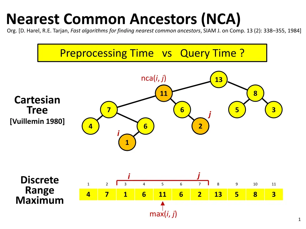
Nearest Common Ancestors (NCA) Org. [D. Harel, R.E. Tarjan, Fast algorithms for finding nearest common ancestors, SIAM J. on Comp. 13 (2): 338 355, 1984] Preprocessing Time vs Query Time ? nca(i, j) 13 8 11 11 Cartesian Tree [Vuillemin 1980] 7 6 5 3 j 2 2 4 6 i 1 1 j i Discrete Range Maximum 1 2 3 4 5 6 7 8 9 10 11 4 7 1 6 11 6 2 13 5 8 3 max(i, j) 1
Cartesian Tree Construction Incremental construction left-to-right 18 18 13 + 13 10 10 8 START HERE 8 2 2 18 13 8 2 10 O(n) time ( = #nodes on rightmost path) 2
Reduction: NCA 1 Discrete Range Maximum nca(i, j) Euler Tour H E E J B F I K A D G G j i C C nca(i, j) j i node H E B A B D C D B E F G F E H J I J K J H depth 2 2 1 2 3 4 3 4 5 4 3 3 4 3 2 1 2 3 2 3 2 1 minimum depth 3
NCA on Perfect Binary Trees 1 2 3 4 5 = nca(11,21) i 11 2i 2i+1 10 20 21 22 23 11 = 10112 21 = 101012 nca(21,21) = 5 = 1012= lcp( 10112 , 101012) longest common prefix proc lcp(x, y) if y < x then swap (x, y) return x >> (msb(x XOR (y >> (msb(y)-msb(x))) position of most significant bit 0 4
Discrete Range Minimum Space O(nlogn) words nca(i, j) 1 1 1 1 3 2 1 1 3 3 4 2 3 2 1 1 2 3 4 3 4 5 4 3 2 3 4 3 j 2 1 2 i 0 1 1 2 3 4 3 4 5 4 3 2 3 4 3 2 1 2 3 3 1 3 3 2 3 3 3 3 2 d 1 1 5 righti drm(i, j) = min(righti(d), leftj(d)) d = msb(i XOR j) leftj 5
Blocked solution Space O(n) words Top structure O(n/log n) elements Space O(n) Query O(1) 1 2 1 2 1 2 3 4 3 4 5 4 1 4 3 4 3 2 3 2 j i block of O(log n) elements Wj(One for each j) 0 1 0 1 1 5 4 3 2 1 Block query: j+1-msb(WjAND ((1 << (j-i+1))-1)) General query: 1 top query + 2 bottom queries O(n) Preprocessing Time O(1) Query Time 6
Summary... General Discrete Range Searching j i 1 2 3 4 5 6 7 8 4 7 1 6 8 6 2 9 Cartesian Tree nca(i, j) 9 8 7 6 NCA j 4 6 2 1 i Discrete Range Max on Depth Array 1 2 3 4 3 4 5 4 3 2 3 4 3 2 1 O(n log n) solution on O(n/log n) blocks O(log n) size blocks O(n) Preprocessing Time O(1) Query Time 7
1d & 2D DRM Results Indexing Model (input accessible) Encoding Model (input not accessable) 2n+o(n) bits, O(1) time [FH07] n/c bits (c) time [BDR10] n/c bits, O(c) time [BDR10] m = 1 1D 2n - O(log n) bits 2n+o(n) bits, O(1) time [F10] (mn log m) bits [BDR10] O(mn log n) bits, O(1) time [BDR10] O(mn log m) bits, O(mn)time[BBD13] O(mn log n) bits, O(1) time [AY10] O(mn) bits, O(1) time [BDR10] mn/c bits (c) time [BDR10] O(c log2c) time [BDR10] O(c log c (loglog c)2) time [BDLRR12] 1<m<n (mn log n) bits [DLW09] O(mn log n) bits, O(1) time [AY10] m = n squared better upper or lower bound ?
DRM encoding - O(n) bits i j A 1 B 2 C 3 D 4 E 5 F 6 G 7 H 8 I J K 11 9 10 nca(i, j) Euler Tour 4 7 1 6 11 6 2 13 5 8 3 H Cartesian Tree E E J B F I K A D G G j i C C nca(i, j) node H E B A B D C D B E F G F E H J I J K J H depth 2 2 1 2 3 4 3 4 5 4 3 3 4 3 2 1 2 3 2 3 2 1 minimum depth select(i) = i th 1 pi j th 1 = select(j) p pj 0 0 0 1 1 0 1 1 0 1 1 1 0 0 1 0 1 1 1 0 0 4n bits + + + + - + + - - - + + - - - + + - + - - rank(p) = drm(i,j) = #1left of p 9 depth = #+- #-= min-prefix-sum(pi,pj)
Succinct data structures for DRM, O(n) bits = log n bits i th 1 = select(i) p 1 0 0 0 0 1 1 0 1 1 0 1 1 1 0 0 1 0 1 1 1 0 0 B3 B0 B1 B2 R1[i] = #1in first i blocks (n/ log n bits) Trank= rank inside block, table lookup (2 +log log bits) rank(p) = R1[ p/ ] + Trank[B[ p/ ], p mod ] +log bits i is in block B[b] leader[i] = is the ith 1 the first 1 in its block? (n bits) rankleader(i) = rank structure for leader array (O(n) bits) Rnonempty= index of nonempty blocks (n/ log n bits) Tselect= select inside block, table lookup (2 +log log bits) PS[b] = #+ - #-for blocks B0..Bb(n/ log n bits) Tps= #+ - #-for block prefix, table lookup (2 +log (1+log ) bits) Tmps= index of minimum prefix sum #+ - #-inside range in a block, table lookup (2 +2log log bits) MPS[b] = PS[b-1]+ Tmps[B[b], 0, -1] (n/ log n bits) drmMPS= drmin structure for MPS, O(n/ ) words (O(n) bits) b2 b1 MPS select(i) = b + Tselect[B[b], i-rank( b-1)] b = Rnonempty[rankleader(i)] min-prefix-sum(pi, pj) = (bk-1)+dk b1= pi/ b3= pj/ b2= drmPS(b1+1, b3-1) d1= Tmps[B[b1], pimod , -1] d2= Tmps[B[b2], 0, -1] d3= Tmps[B[b3], 0, pjmod ] k = argmint=1..3PS[bt-1]+Tps[B[bt], dt] b3 1 3 2 1 2 1 d3=1 d1=3 pj d2=2 pi + + + + - + + - - - + + - - - + + - + - - 10 Bb1 Bb2 Bb3
")


 words")
 words")


 bits")
 bits")