Finite Difference Method for Conductive Heat Flow in Solids
Illustrated with examples, the finite difference method is applied to analyze 2D time-independent conductive heat flow in solids. The conservation of heat energy, temperature variation in heat-conducting solids, and boundary conditions are discussed in detail. Emphasis is placed on solution techniques for dynamical problems using matrix calculations and satisfying equations at boundary points.

Download Presentation

Please find below an Image/Link to download the presentation.
The content on the website is provided AS IS for your information and personal use only. It may not be sold, licensed, or shared on other websites without obtaining consent from the author.If you encounter any issues during the download, it is possible that the publisher has removed the file from their server.
You are allowed to download the files provided on this website for personal or commercial use, subject to the condition that they are used lawfully. All files are the property of their respective owners.
The content on the website is provided AS IS for your information and personal use only. It may not be sold, licensed, or shared on other websites without obtaining consent from the author.
E N D
Presentation Transcript
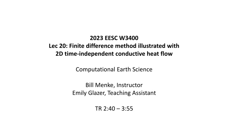
2023 EESC W3400 Lec 20: Finite difference method illustrated with 2D time-independent conductive heat flow Computational Earth Science Bill Menke, Instructor Emily Glazer, Teaching Assistant TR 2:40 3:55
Today New (and fairly technical) Stuff Finite Difference Method for Solving Dynamical Problems
Today all Lecture Thursday all in-class projects so be sure to attend
Example of Temperature variation in heat-conducting solid in the equilibrium approximation (meaning no time dependence)
Conservation of heat energy ? ??? ??+??? ?? ??= ?? ?? ?? and ? + ? ?? increase in heat ?? net flux in heat source
??? ??+??? ?? ??= + ? ?? ?? ?? ?? and ? heat proportional to temperature ? = ???? ??= ??? ?? ?? heat flows from hot to cold ??= ??? ??
??? ??+??? ?? ??= + ? ?? ? = ???? ??= ??? ?2? ??2+?2? ?? ??= ? ??? + ? ?? ??2 ??= ??? ??
?2? ??2+?2? ?? ??= ? ??? + ? ??2 ? = ?/? at equilibrium ?? ??=0 ?2? ??2+?2? ??2= ?
boundary ? = ???? boundary ? = ???? boundary ? = ???? Inside ?2? ??2+?2? ??2= ? boundary ? = ????
at every boundary point ? is specified at every boundary point ? is specified at every boundary point ? is specified at every inside point equation is satisfied at every boundary point ? is specified
only consider points on a ?? ?? grid use matrix ??? for ? ??,?? values
obey top BC obey left BC obey right BC obey bottom BC obey equation
? obey top BC ?00= ???? ?10= ???? ?20= ???? ? ?? equations
? obey left BC ?00= ????? ?01= ????? ?11= ????? ? ?? 2 equations
? ? obey equation ??? in interior obeys the equation ? ? ???= ? ?? 2 ?? 2 equations
?2? ??2+?2? ? + 1 at ??,?? ??2= ? ? ?? ???+ ,? 1 ??= ??+1,? ??,? ? ?
?2? ??2+?2? at ??,?? ??2= ? ? 1 ? ?? ???+ ,? 1 ??= ??+1,? ??,? ? ? ?? ??? ,? 1 ??= ??,? ?? 1,? ?
?2? ??2+?2? at ??,?? ??2= ? ? ?? ???+ ,? 1 ??= ??+1,? ??,? ? ? ?? ??? ,? 1 ??= ??,? ?? 1,? ? ?2? ??2 1 ?? ?? ?
?2? ??2+?2? at ??,?? ??2= ? ?2? ??2 1 ?2?? 1,? 2??,?+ ??+1,?
?2? ??2+?2? at ??,?? ??2= ? ?2? ??2 1 ?2??,? 1 2??,?+ ??,?+1
?2? ??2+?2? at ??,?? ??2= ? = ???
?2? ??2+?2? at ??,?? ??2= ? 1 1 ?2?? 1,? 2??,?+ ??+1,? + ?2??,? 1 2??,?+ ??,?+1 = ??? ?? 1,? ?2 2??,? ?2+??+1,? ??,? 1 ?2 2??,? ?2+??,?+1 + = ??? ?2 ?2 ?? 1,? ?2+??+1,? ?2??,?+??,? 1 ?2+??,?+1 2 2 ?2 ?2+ ?2= ???
?2? ??2+?2? at ??,?? ??2= ? ? equation at ??,?? involves 5 points ? ?? 1,? ?2+??+1,? ?2??,?+??,? 1 ?2+??,?+1 2 2 ?2 ?2+ ?2= ???
number of unknown Temperature values: ? = ?? ?? number of equations 2?? top & bottom +2 ?? 2 left and right + ?? 2 ?? 2 interior
number of unknown Temperature values: ? = ?? ?? number of equations 2?? 2?? top & bottom +2?? 4 +2 ?? 2 left and right +???? 2?? 2??+ 4 + ?? 2 ?? 2 interior = ????= ?
number of unknown Temperature values: ? = ?? ?? number of equations ? = ?? ?? number of unknown equal number of equations ? = ? suggests problem is solvable
Solution method write down matrix equation of the form ?? = ?for unknown ???s every equation (boundary or interior) is a row and solve the equation
Logistical issue #1 whereas the matrix equation ?? = ?has unknown vector? unknown temperatures are a matrix?
? ? ? ? ? ? ? ? ? Solution to Logistical issue #1 unwrap the matrix ? into a vector ? ? ? ? ? ? ? ? ? ?
? ? ? ? ? ? ? ? ? ? ? ? ? ? ? ? ? ? creates quite a bookkeeping problem!
? ? ? ? ? ? ? ? ? ? ? ? ? ? ? ? ? ? ? simplified by lookup tables ? i=iofk[k,0]; j=jofk[k,0]; k=kofij[i,j]; ? creates quite a bookkeeping problem!
# lookup tables translate between matrix (i,j) # and vector ordering k M= Lx*Ly; iofk = np.zeros((M,1),dtype=int); jofk = np.zeros((M,1),dtype=int); kofij = np.zeros((Lx,Ly),dtype=int); k=0; for ix in range(Lx): for iy in range(Ly): iofk[k,0]=ix; jofk[k,0]=iy; kofij[ix,iy]=k; k=k+1;
Logistical issue #2 the matrix ? in the matrix equation ?? = ?is huge ??= ??= 100 ? = ? = ?? ??= 10,000 ? 10,000 10,000 ? 100,000,000 elements ?
Solution to Logistical issue #2 define ? as a sparse matrix so that only it non-zero elements are stored ? fortunately most of them are zero 10,000 10,000 ? in our case, ? no more than 5 per row
Steps to making a sparse matrix D (1)create three vectors Dr, Dc and Dv to hold the row-index, column-index, and value of non-zero elements of D (2) For each non-zero elements of D, set one row of Dr, Dc and Dv (3) Call a Python method that creates the sparse matrix
?? ?? ?=5 ?? ? = 4 ?.? 5 4 ?.? ?
(1)create the three vectors Pmax = 100000; maximum number of non-zero elements
Pmax = 100000; Dr = np.zeros((Pmax,1),dtype=int); Dc = np.zeros((Pmax,1),dtype=int); row and column vectors must be integer
Pmax = 100000; Dr = np.zeros((Pmax,1),dtype=int); Dc = np.zeros((Pmax,1),dtype=int); Dv = np.zeros((Pmax,1)); value vector
Pmax = 100000; Dr = np.zeros((Pmax,1),dtype=int); Dc = np.zeros((Pmax,1),dtype=int); Dv = np.zeros((Pmax,1)); s = np.zeros((M,1)); RHS vector of ?? = ?
(2) For each non-zero elements of D, set one row of Dr, Dc and Dv nr=0; counter for the rows of D every point in the grid is a different row
nr=0; ne=0; counter for the non-zero elements of D
nr=0; ne=0; mel=0; mer=0; meb=0; met=0; mi=0; counters for the number of left, right, bottom, top and interior points
nr=0; ne=0; mel=0; mer=0; meb=0; met=0; mi=0; for ix in range(Lx): for iy in range(Ly): loop over all the grid points [code here to set the elements of one row at a time of D]
# left boundary point if( (ix==0) and (iy>0) and (iy<(Ly-1))): test whether this (ix,iy) in on the left boundary
# left boundary point if( (ix==0) and (iy>0) and (iy<(Ly-1))): k=kofij[ix,iy]; convert (ix,iy) of D into a k of m
# left boundary point if( (ix==0) and (iy>0) and (iy<(Ly-1))): k=kofij[ix,iy]; mel=mel+1;this is a left element, so increment the left-element counter
# left boundary point if( (ix==0) and (iy>0) and (iy<(Ly-1))): k=kofij[ix,iy]; mel=mel+1; Dr[ne,0] = nr; Dc[ne,0] = k; Dv[ne,0] = 1.0; Define this non-zero element row of D col of D value of D
# left boundary point if( (ix==0) and (iy>0) and (iy<(Ly-1))): k=kofij[ix,iy]; mel=mel+1; Dr[ne,0] = nr; Dc[ne,0] = k; Dv[ne,0] = 1.0; ne=ne+1; increment the element counter
# left boundary point if( (ix==0) and (iy>0) and (iy<(Ly-1))): k=kofij[ix,iy]; mel=mel+1; Dr[ne,0] = nr; Dc[ne,0] = k; Dv[ne,0] = 1.0; ne=ne+1; s[k,0]=ExLeft[iy-1,0]; set the RHS vector


")


create the three vectors")


 For each non-zero elements of D, set one row of Dr, Dc")