Finite Element Discretization for Structural Domain Equations
Explore figures depicting numerical solutions, exact solutions, and finite element discretizations for structural domain equations. Understand concepts such as approximate solutions, interpolated solutions, and gradients, with comparisons between exact and approximate values.

Download Presentation

Please find below an Image/Link to download the presentation.
The content on the website is provided AS IS for your information and personal use only. It may not be sold, licensed, or shared on other websites without obtaining consent from the author. If you encounter any issues during the download, it is possible that the publisher has removed the file from their server.
You are allowed to download the files provided on this website for personal or commercial use, subject to the condition that they are used lawfully. All files are the property of their respective owners.
The content on the website is provided AS IS for your information and personal use only. It may not be sold, licensed, or shared on other websites without obtaining consent from the author.
E N D
Presentation Transcript
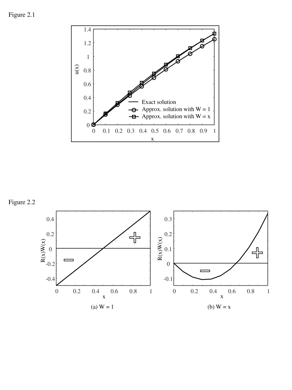
Figure 2.1 1.4 1.2 1 u(x) 0.8 0.6 0.4 Exact solution Approx. solution with W = 1 Approx. solution with W = x 0.2 0 0 0.1 0.2 0.3 0.4 0.5 0.6 0.7 0.8 0.9 x 1 Figure 2.2 0.4 0.3 0.2 0.2 R(x)W(x) R(x)W(x) 0 0.1 -0.2 0 -0.4 -0.1 0 0.2 0.4 0.6 0.8 1 0 0.2 0.4 0.6 0.8 1 x x (a) W = 1 (b) W = x
Figure 2.3 1.6 1.4 1.2 u(x), du/dx 1 0.8 uexact uapprox duexact/dx duapprox/dx 0.6 0.4 0.2 0 0 0.2 0.4 0.6 0.8 1 x Figure 2.4 0.1 0.05 0 u(x), du/dx -0.05 uexact uapprox duexact/dx duapprox/dx -0.1 -0.15 -0.2 -0.25 0 0.2 0.4 0.6 0.8 1 x
4 Figure 2.5 3 2 wexact wapprox wexact wapprox w, w 1 0 -1 -2 0 0.2 0.4 0.6 0.8 1 x Figure 2.6 F t s xy y xx x + + = 0 b x Structure t s xy x yy y + + = 0 b y (a) Structural domain with governing differential equations F Element (b) Finite element discretization
Figure 2.7 u(x) Nodes Approximate solution x Finite elements Exact solution Figure 2.8 u Exact solution Two elements Four elements Eight elements x n 1 1 2 n Figure 2.9 n 1 n+1 n 1 2 3 ui+1 ui i+1 i xi L(i) xi+1
Figure 2.10 u ui+2 d d u x ui ui+1 xi xi+1 xi+2 xi xi+1 xi+2 (a) Interpolated solution (b) Gradient of solution Figure 2.11 1 ( ) f ix - 1 i ( ) 1/ L xi+1 xi 2 xi xi 1 ( ) i - 1/ L ( ) x d f i dx Figure 2.12 1.0 1(x) 2(x) 3(x) (x) 0.5 0 0.5 x 1.0 0
Figure 2.13 1.6 1.2 u(x) 0.8 u-exact u-approx. 0.4 0 0 0.2 0.4 0.6 0.8 1 x 2 Figure 2.14 1.5 1 du/dx du/dx (exact) du/dx (approx.) 0.5 0 0 0.2 0.4 0.6 0.8 1 x 1( ) 2( ) x N x N Figure 2.15 Element e i x j x x ( ) e L
Figure 2.16 0.08 u-approx. u-exact 0.06 u(x) 0.04 0.02 0 0 0.2 0.4 0.6 0.8 1 x Figure 2.17 F3 F2 3 2 r r 1 4 F1 F4 Equilibrium Virtual displacement Figure 2.18 xu x u mg mg
Figure 2.19 x E, A(x) F Bx L u2 Figure 2.20 F3 1 3 2 1 F3 3 2 u3 u1 bx Figure 2.21 F u1 u2 u3 Figure P2.17 1 2 3 1 m 1 m x Figure P2.18 x f L
Figure P2.19 x E A L q Figure P2.20 L = 1 m Figure P2.21 0.3 106 N 0.3 m Figure P2.22 RL RR F 0.3 m 0.4 m 0.3 m q Figure P2.23 LT q = cx E, A Figure P2.26 L x, u
Figure P2.27 y 1 2 x x = 1 x = -1 u1 u2 u3 Figure P2.28 1 2 3 1/4 3/4 x u1 u2 u3 1 2 3 x = -1 x = 0 x = 1 q x


