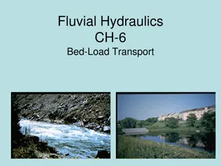
Fluvial Hydraulics CH-6

This content delves into the intricate calculations and methods involved in total load transport in fluvial hydraulics. It discusses the total bed-material load, wash load, different equations for bed-load transport, indirect and direct methods, parameters proposed by Graf et al. and Ackers and White, as well as evaluations from various experiments. Insightful visuals accompany the detailed explanations provided, making it a comprehensive resource for understanding total load transport phenomena in hydraulic systems.

Download Presentation

Please find below an Image/Link to download the presentation.
The content on the website is provided AS IS for your information and personal use only. It may not be sold, licensed, or shared on other websites without obtaining consent from the author.If you encounter any issues during the download, it is possible that the publisher has removed the file from their server.
You are allowed to download the files provided on this website for personal or commercial use, subject to the condition that they are used lawfully. All files are the property of their respective owners.
The content on the website is provided AS IS for your information and personal use only. It may not be sold, licensed, or shared on other websites without obtaining consent from the author.
E N D
Presentation Transcript
Fluvial Hydraulics CH-6 Total Load Transport
Total Load Total Load = total bed-material load + wash load Wash load is commonly neglected In fact, Graf refers more to total load transport as being total bed-material load transport We have already derived Einstein s equation for total bed- material load: = + = i q i q i q i q sb sb ss ss sb sb s s h + + 1 . 2 303 log 30 2 . I I 1 2 Note: for non-uniform sediments, two options: Calculate for each grain size and sum over all fractions Use equivalent diameter (d35)
Total Bed-Load Transport Equations Indirect Methods: determine bed-material load by addition of the calculated bed load and calculated suspended load Different hydrodynamics of each mode of transport Einstein s method Direct Methods: determine bed-material load directly without making a distinction between two modes of transport
Direct Total Bed-Load Transport Equations Graf et al. (1968): Defined parameter of shear intensity: 1 ) 1 ( h e R S s d = = s A * Proposed a parameter of transport: q UR s q C UR h = = s h gd ( ) ( ) A 3 3 1 1 s s gd s s = volumetric concentrat ion C s = d d 50 Functional relationship exists between these two parameters: ( ) A A fct =
Direct Total Bed-Load Transport Equations Graf et al. (1968): Used some 800 experiments from laboratory and 80 experiments in the field: ( ) 10 10 A or for . 2 52 = 10 . 39 A A 2 3 14 6 . A Graf et al. (1987) evaluated above relationship and suggested slightly modified form: ( ) 4 . 10 = A A K 5 . 1 = K A K A 1 14 6 . if ( 0 ) 5 . 2 = 1 . 0 if 045 22 2 . 14 6 . if A A = 22 2 . K A
Direct Total Bed-Load Transport Equations Ackers and White (1973): Proposed parameter of mobility of sediments: n u F 1 ( ) n w U w = * ( ) gr 10 h 1 s gd 32 log m s d = = 1 F for n * gr w Proposed a parameter of transport of sediments: m F w gr = 1 G C gr w A w Total-load transport becomes q C = n w d U = s G s gr q h u * m
Direct Total Bed-Load Transport Equations Ackers and White (1973): Note: hm= A/B (average flow depth) Coefficients in above relations determined by regression analysis (1000 experiments in lab and 250 experiments in field): Range of validity: 0.04 < d50[mm] < 4.0 and Fr < 0.8 For non-uniform material, use d = d35
Evaluation of Total Bed-Material Load Transport Equations White et al. (1973) compared over 19 equations with experimental results from 1000 lab experiments and 270 field experiments: Lab: 0.04 < d50[mm] < 4.9 and h < 0.4 m Field: 0.1 < d50[mm] < 68.0 and 9 < B/h < 160 Approximately 10 formulas had success rates of less than 40%
Evaluation of Total Bed-Material Load Transport Equations Conclusion is that these formulas give guidance to engineer (not true value) Advised to consult more than one formula and consider potential range in transport rates
Wash Load Component Wash Load (qsw) particles that are never in contact with the bed (washed through the channel by the flow) Limited to very finest particles which make up very small portion of the bed material Distribution of particles rather uniform over the entire flow depth Attempts to define wash load component: Einstein (1950) wash load corresponds to fraction of PSD smaller than 10% Raudkivi (1976) particles with diameter less than 0.06 mm No physical relationship to flow No analytical method In order to obtain quantitative information on wash load, measurements in the field must be performed Measures qss+ qsw To get qsw, you must then calculate qssand back calculate qsw Graf: When wash load is a greater contributor to total sediment load (qsw > qsw), the problem of sediment transport becomes hopelessly complicated
Graf Example 6.F We established the stage-discharge curve for a range of 10 < Q [m3/s] < 1000 for a river in an earlier example (remember the first use of the Einstein-Barbossa curve). The width of the river is 90 m, bed slope is 0.0005, and the non- erodible banks have a slope of 1:1. Sediment forming the bed has a ss= 2.65, d50= 0.32 mm, d35= 0.29 mm, and d90= 0.48 mm. Water temperature is 14oC. Determine the stage/sediment-discharge curve (sedimentological rating curve) using Einstein, Graf et al. (1968) and Ackers and White methods.