Fourier Analysis of Continuous-Time Systems in Electrical Engineering

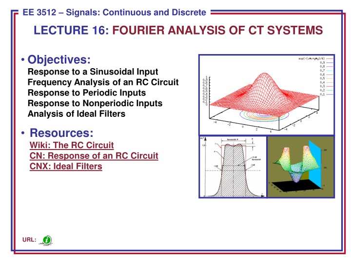
ECE 8443 Pattern Recognition EE 3512 Signals: Continuous and Discrete LECTURE 16: FOURIER ANALYSIS OF CT SYSTEMS Objectives: Response to a Sinusoidal Input Frequency Analysis of an RC Circuit Response to Periodic Inputs Response to Nonperiodic Inputs Analysis of Ideal Filters Resources: Wiki: The RC Circuit CN: Response of an RC Circuit CNX: Ideal Filters URL:

Differential Equations For CT systems, such as circuits, our principal tool is the differential equation. For the circuit shown, we can easily compute the input/output differential equation using Kirchoff s Law. What is the nature of the impulse response for this circuit? + = ( ) ( ) ( ) 0 dy Ri t y t x t ( ) dv t ( ) t = = C ( ) i t C C dt dt ( ) dy t + = ( ) ( ) 0 RC y t x t dt ( ) 1 1 dy t + = ( ) ( ) y t x t dt RC RC EE 3512: Lecture 16, Slide 1

Numerical Solutions to Differential Equations We can replace n by n-1 to obtain: ) 1 ( ] [ = y aT n y Consider our 1st-order diff. eq.: ) ( t ay dt dy t ] 1 + ] 1 [ [ n bTx n = + ( ) ( ) bx t This is called the Euler approximation to the differential equation. We can solve this numerically by setting t = nT: ) ( nT ay dt nT t = =0 dy t [ ] With and initial condition, , the solution is: ] 0 [ y = y aT n y x n n = + ( ) ( ) bx nT The derivative can be approximated: nT y dt nT t = = n [ ] 1 ( ) 0 [ ], , 1 , 0 , 2 ... n + ( ) ( ) ( ) dy t T y nT The CT solution is: = t y = T at ( ) 0 ( y ), 0 e t Substituting into our diff. eq.: ( ) ( T [ ) ( n x nT x = + ) y nT T y nT Later, we will see that using the Laplace transform, we can obtain: 0 [ ] [ = y e n y = + ( ) ( ) ay nT bx nT = Let and : ] ( ) [ ] y nT y n = anT ], , 1 , 0 , 2 ... n But we can approximate this: + [ ] 1 T [ ] y n y n = + [ ] [ ] ay n bx n 2 2 3 3 a T a T = + + aT 1 ... e aT 2 6 ] 1 + = + [ [ ] [ ] [ bTx ] y n y n aTy n bTx n Which tells us our 1st-order approximation is accurate! ] 1 + = + [ 1 ( ) [ ] [ ] y n aT y n n EE 3512: Lecture 16, Slide 2

Higher-Order Derivatives We can use the same approach for the second-order derivative: ( ) ( ) dy t dy t dt dt 2 ( ) d y t = = + = t nnT T t nnT dt T = t nT + + + ( 2 ) 2 ( ) ( ) y nT T y nT T y nT = T Higher-order derivatives can be similarly approximated. Arbitrary differential equations can be converted to difference equations using this technique. There are many ways to approximate derivatives and to numerically solve differential equations. MATLAB supports both symbolic and numerical solutions. Derivatives are quite tricky to compute for discrete-time signals. However, in addition to the differences method shown above, there are powerful methods for approximating them using statistical regression. Later in the course we will consider the implications of differentiation in the frequency domain. EE 3512: Lecture 16, Slide 3

Series RC Circuit Example ( ) 1 1 dy t + = ( ) ( ) y t x t dt RC RC Difference Equation: R=1;C=1;T=0.2; a=-(1-T/R/C);b=[0 T/R/C]; y0=0; x0=1; n=1:40; x=ones(1,length(n)); y1=recur(a, b, n, x, x0, y0); Analytic Solution: t=0:0.04:8; y2=1-exp(-t); y1=[y0 y1]; n=0:40; plot(n*T, y1, o , t, y2, - ); EE 3512: Lecture 16, Slide 4

Example: RC Circuit ( ) 1 1 dy t + = ( ) ( ) y t x t dt RC RC Using our FT properties: 1 1 ( ) ( ) + = ( ) j Y Y X RC / 1 RC RC / 1 + ( ) ( = ) Y X j RC ( ) / 1 Y RC / 1 + ( = = ) H ( ) X j RC / 1 + RC ( = ) H 2 2 / 1 ( ) RC ( ) ( = 1 ) tan H RC Compute the frequency response: RC = 0.001; W=0:50:5000; H=(1/RC)./(j*w+1/RC); magH=abs(H); angH=180*angle(H)/pi; EE 3512: Lecture 16, Slide 5

Response of an LTI System to a Sinusoid Consider an LTI CT system with impulse response h(t): = = ( d ( ) ( ) * ( ) ) ( ) y t h t x t h x t We will assume that the Fourier transform of h(t) exists: j ( = t ) ( ) H h t e dt The output can be computed using our Fourier transform properties: ( ) ( and ) ( ) ( ) ( H Y X H Y = = = + ) ( ) ( ) ( ) ( ) X Y H X Suppose the input is a sinusoid: cos( ) ( 0 + = t A t x ) Using properties of the Fourier transform, we can compute the output: ( ) ( ) ( ) ( ) ( e e H A + + = ) j j = + + ( ) X A e e 0 0 = Y H X j ( ) ( ) j j = + + ( ) 0 0 ( ) ( ) j ( ) ( + ) A H e H e + 0 0 0 0 ( ) ( ) ( ) ( ) j j = ( ) ( ) j H j H ( ) A H e e e e 0 0 0 0 + 0 )( ) )( ) ( ( + + = + ( ) ( ) j H j H ( ) A H e e 0 0 0 0 0 ( ) ( ) ) 0 = = + + 1 - F ( ) ( ) ( ) cos ( y t Y A H t H 0 0 EE 3512: Lecture 16, Slide 6

Example: RC Circuit (Cont.) We can compute the output for RC=0.001 and 0=1000 rad/sec: ( ) + = 45 1000 cos ) 707 . 0 ( ) ( t A t y We can compute the output for RC=0.001 and 0=3000 rad/sec: ( + = 6 . 71 3000 cos ) 316 . 0 ( ) ( t A t y ) Hence the circuit acts as a lowpass filter. Note the phase is not linear. If the input was the sum of two sinewaves: ( ) ( t t x 3000 cos 100 cos ) ( + = ) t describe the output. EE 3512: Lecture 16, Slide 7

Response To Periodic Inputs We can extend our example to all periodic signals using the Fourier series: ( ) variant (a cos ) ( 1 = k 0 = + + of the trigonome tric Fourier series) x t a A k t 0 k k The output of an LTI system is: ( ) + = 0 0 ) ( H a t y ( ) ( ( ) ) k + + cos A H k k t H k 0 0 0 k k 1 We can write the Fourier series for the output as: ( cos ) ( 1 k = ) = + k + y y y y t a A t 0 0 k k where, = = k = + k y 0 x y x k y x a ) 0 ( H ( ) ( ) a A A H H 0 0 0 k k k also, 1 = k = + k y k y k x k x c ( ) and c ( ) A H H 0 0 k 2 It is important to observe that since the spectrum of a periodic signal is a line spectrum, the output spectrum is simply a weighted version of the input, where the weights are found by sampling of the frequency response of the LTI system at multiples of the fundamental frequency, 0. EE 3512: Lecture 16, Slide 8

Example: Rectangular Pulse Train and an RC Circuit Recall the Fourier series for a periodic rectangular pulse: ( ) = + k ( ) cos x t a a t 0 k 1 k where, ( k ) k sin / 2 = = 5 . 0 a a 0 k ( ) 2 / / 1 RC / 1 + = Also recall the system response was: ( ) H j RC The output can be easily written as: where, ( ) = + + y y y ( ) cos y t a A k t 0 0 k k 1 k = = y 0 x ) 0 ( H 5 . 0 a a 0 ( ) sin / 2 / 1 k RC = = y x k ( ) A A H k 0 k ( ) 2 / k + 2 2 ( ) / 1 ( ) k RC 2 / 1 RC odd k = k + 2 2 ( ) / 1 ( ) k RC 0 even k EE 3512: Lecture 16, Slide 9

Example: Rectangular Pulse Train (Cont.) We can write a similar expression for the output: = odd k ( ) 2 / 1 RC = + RC 1 y 0 ( ) cos tan y t a k t k k + 2 2 ( ) / 1 ( ) k RC 1 k 1/RC = 1 We can observe the implications of lowpass filtering this signal. What aspects of the input signal give rise to high frequency components? 1/RC = 10 What are the implications of increasing 1/RC in the circuit? Why are the pulses increasingly rounded for lower values of 1/RC? 1/RC = 100 What causes the oscillations in the signal as 1/RC is increased? EE 3512: Lecture 16, Slide 10

Response to Nonperiodic Inputs We can recover the output in the time domain using the inverse transform: 2 1 j j j = d t ( ) ( ) ( ) y t H e X e e These integrals are often hard to compute, so we try to circumvent them using transform tables and combinations of transform properties. Consider the response of our RC circuit to a single pulse: ) 2 / sin( ) ( = j X e ( ) 2 / / 1 RC / 1 + = j ( ) H e j RC = j j j ( ) ( ) ( ) Y e X sin( e H ) 2 / e / 1 RC / 1 + = ( ) 2 / j RC MATLAB code for the frequency response: RC=1; w=-40:.3:40; X=2*sin(w/2)./w; H=(1/RC)./(j*w+1/RC); Y=X.*H; magY=abs(Y); EE 3512: Lecture 16, Slide 11

Response to Nonperiodic Inputs (Cont.) We can recover the output using the inverse Fourier transform: syms X H Y y w X = 2*sin(w/2)./w; H=(1/RC)./(j*w+1/RC); Y=X.*H; Y=ifourier(Y); ezplot(y,[-1 5]); axis([-1 5 0 1.5]) 1/RC = 1 1/RC = 1 1/RC = 10 1/RC = 10 EE 3512: Lecture 16, Slide 12

Ideal Filters The process of rejecting particular frequencies or a range of frequencies is called filtering. A system that has this characteristic is called a filter. An ideal filter is a filter whose frequency response goes exactly to zero for some frequencies and whose magnitude response is exactly one for other ranges of frequencies. To avoid phase distortion in the filtering process, an ideal filter should have a linear phase characteristic. Why? passband filter the in all for ) ( d t e H = j We will see this ideal response has some important implications for the impulse response of the filter. Highpass Lowpass Bandstop Bandpass EE 3512: Lecture 16, Slide 13

Ideal Linear Phase Lowpass Filter Consider the ideal lowpass filter with frequency response: Phase Response B , j dt , e B B = j ( ) H e 0 B Using the Fourier transform pair for a rectangular pulse, and applying the time-shift property: Impulse Response B B = ( ) sin ( h t c t dt Is this filter causal? The frequency response of an ideal bandpass filter can be similarly defined: = elsewhere , 0 j dt , e B B j 1 2 ( ) H e Will this filter be physically realizable? Why? EE 3512: Lecture 16, Slide 14

Summary Showed that the response of a linear LTI system to a sinusoid is a sinusoid at the same frequency with a different amplitude and phase. Demonstrated how to compute the change in amplitude and phase using the system s Fourier transform. Demonstrated this for a simple RC circuit. Generalized this to periodic and nonperiodic signals. Worked examples involving a periodic pulse train and a single pulse. Introduced the concept of an ideal filter and discussed several types of ideal filters. Noted that the ideal filter is a noncausal system and is not physically realizable. However, there are many ways to approximate ideal filters, and that is a topic known as filter design. EE 3512: Lecture 16, Slide 15