Gabor Transform: Definitions, Approximations, and Applications

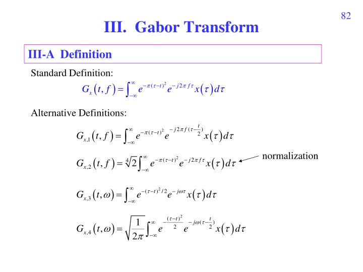
82 III. Gabor Transform III-A Definition Standard Definition: ( ) ( ) = 2 ( ) 2 t j f , G t f e e x d x Alternative Definitions: t 2 ( ) j f ( ) ( ) = 2 ( ) t ,1 , G t f e e x d 2 x normalization ( ) ( ) 2 = ( ) 2 t j f 4 , 2 G t f e e x d ,2 x ( ) ( ) = 2 ( ) /2 t j , G t e e x d ,3 x 2 ( ) t t 1 ( ) j ( ) ( ) = , G t e e x d 2 2 ,4 x 2

83 Main Reference S. Qian and D. Chen, Sections 3-2 ~ 3-6 in Joint Time-Frequency Analysis: Methods and Applications, Prentice-Hall, 1996. Other References D. Gabor, Theory of communication , J. Inst. Elec. Eng., vol. 93, pp. 429-457, Nov. 1946. ( Gabor transform) M. J. Bastiaans, Gabor s expansion of a signal into Gaussian elementary signals, Proc. IEEE, vol. 68, pp. 594-598, 1980. R. L. Allen and D. W. Mills, Signal Analysis: Time, Frequency, Scale, and Structure, Wiley- Interscience. S. C. Pei and J. J. Ding, Relations between Gabor transforms and fractional Fourier transforms and their applications for signal processing, IEEE Trans. Signal Processing, vol. 55, no. 10, pp. 4839-4850, Oct. 2007.

84 Note Gabor transform short-time Fourier transform (STFT) Gabor transform STFT special case.

85 III-B Approximation of the Gabor Transform Although the range of integration is from to , due to the fact that 2 a when |a| > 1.9143 0.00001 e 2/2 e when |a| > 4.7985 a 0.00001 the Gabor transform can be simplified as: 1.9143 + t ( ) ( ) 2 ( ) 2 t j f , G t f e e x d x 1.9143 t 2 ( ) t t 1 + ( ) 4.7985 j t ( ) ( ) = , G t e e x d 2 2 ,3 x 2 4.7985 t

86 III-C Why Do We Choose the Gaussian Function as a Mask (1) Among all functions, the Gaussian function has the advantage that the area in time-frequency distribution is minimal. ( STFT time-domain frequency domain ) w(t) time domain w(t) W(f) = FT[w(t)] frequency domain (2) Special relation between the Gaussian function and the rectangular function

87 (Note): Gaussian function FT eigenfunction Gabor transform time domain frequency domain 2 2 = 2 t j f t f e e dt e 2 2 j t = /2 /2 t f e e dt e 2 2 + = a e ( ) /4 at bt b a / e dt according to M. R. Spiegel, Mathematical Handbook of Formulas and Tables, McGraw-Hill, 3rdEd., 2009. Gaussian function is also an eigenmode in optics, radar system, and other electromagnetic wave systems. (will be illustrated in the 8thweek)

88 Uncertainty Principle (Heisenberg, 1927) For a signal x(t), if when |t| , then ( ) t x t = 0 t f 1/4 ( ) ( ) f df where , t = = 2 2 2 f 2 ( ) ( ) , t P t dt f P t x f X = ( ) = ( ) f df f P , t P t dt f X t x 2 | ( )| | ( )| x t x t 2 ( ) | ( )| ( )| X f X f = , P t ( ) f = , P x 2 dt X 2 | df

89 (Proof of Henseinberg s uncertainty principle): From simplification, we consider the case where t= f= 0 Then, use Parseval s theorem ( )| 2 2 2 | ( )| x t | t dt x t dt 1 = 2 t 2 f 2 4 2 2 | ( )| x t | ( )| x t dt dt = 2 2 | ( )| x t | ( )| X f dt df if X(f) = FT[x(t)]

90 2 ( ), ( ) x t x t ( ), ( ) y t y t ( ), ( ) x t y t From Schwarz s inequality 2 2 d dt d dt ( ) ( ) ( )| x t + 2 2 2 | ( )| x t | ( ) x t dt ( ) /2 t dt dt tx t tx t x t dt 2 d dt d dt ( ) ( ) (using |a+b|2+ |a b|2 2|a|2) + ( ) x t ( ) /4 tx t tx t x t dt 2 d dt 2 = = ( ) x t x t ( ) /4 ( ) ( ) ( ) ( ) x t x t dt /4 t dt tx t x t 2 = ( ) ( ) ( ) ( ) ( ) ( ) x t x t dt /4 tx t x t tx t x t t t 2 2 = ( ) x t /4 dt 1 1 2 t 2 f t f 2 16 4

91 For Gaussian function ( ) x t ( ) 2t 2 = = f e X f e ) | ( )| x t 2 2 2 2 ( | ( )| x t t dt t dt ( ) t = = = 2 t 2 ( ) t P t dt t x 2 2 | ( )| x t | ( )| x t dt dt t = 0 Since ( ) x t 2 2 = = 2 t ? dt e dt 2 2 + = a e ( ) /4 at bt b a / e dt use ( ) 3/ 2 1 ( ) 2 2 2 = = = = 2 2 2 2 2 t t 2 22(2 ) t x t dt t e dt t e dt 3/2 5/2 2 0 + [( 2 ) 1 1)/2] m a = 2 = use m at t e dt 1)/2 + ( m 0 ( ( ) n ( ) ( ) + = = , 3/ 2 / 2 n n 1/2

92 2 2 | ( )| x t t dt 1, 4 1 = = 2 t t = 2 | ( )| x t dt 4 1 = , f 4 Gaussian function 1 = t f 4 [ ] M. R. Spiegel, Mathematical Handbook of Formulas and Tables, McGraw-Hill, 3rdEd., 2009.

93 III-D Simulations Gabor transform for Gaussian function exp( t2) rec-STFT, B = 0.5 for Gaussian function exp( t2) 4 4 3 3 2 2 1 1 f-axis f-axis 0 0 -1 -1 -2 -2 -3 -3 -4 -4 -4 -3 -2 -1 t-axis 0 1 2 3 4 -4 -3 -2 -1 0 1 2 3 4 t-axis

94 x(t) = cos(2 t) when t < 10, x(t) = cos(6 t) when 10 t < 20, x(t) = cos(4 t) when t 20 Gabor 5 4 3 2 Frequency (Hz) 1 0 -1 -2 -3 -4 -5 0 5 10 15 20 25 30 Time (Sec)

95 Gabor transform of s(t) Gabor transform of r(t) 4 4 3 3 2 2 1 1 f-axis f-axis 0 0 -1 -1 -2 -2 -3 -3 -4 -4 -10 -5 0 5 10 -10 -5 0 5 10 t-axis t-axis ( ) ( ) s t s(t) = 0 otherwise, = 2 exp /10 3 jt j t for 9 t 1, ( ) ( ) r t = + 2 2 exp /2 6 exp j t ( 4) /10 jt t

96 Gabor transform for s(t) + r(t) 4 3 2 1 f-axis 0 -1 -2 -3 -4 -10 -5 0 5 10 t-axis

97 III-E Properties of Gabor Transforms ( ) ( ) = 2 2 ( ) j f t , G t f e e x d x (1) Integration property ( ) ( ) 2 2 t When k 0, = ( ) 0 2 ( 1) j kt f k , G t f e ( , x G t f df df e x kt x ) 2 = t e x When k = 0, When k = 1, (recovery property) ( ) , x G t f e ( ) x t = 2 j t f df (2) Shifting property ( ) ( ) = 2 j f t If y(t) = x(t t0), then . (3) Modulation property , , G t f G t t f e 0 0 y x ( ) ( ) If y(t) = x(t)exp(j2 f0t), then = , , G t f G t f f 0 y x

98 (4) Special inputs: ( ) (a) When x( ) = ( ), 2 = t , G t f e x ( ) 2 (b) When x( ) = 1, = 2 j f t f , G t f e e x (symmetric for the time and frequency domains) f f t t

99 (5) Power decayed property If x(t ) = 0 for t > t0, then . ( ) , x G t f df ( ) 2 2 2 2 ( t t ) , e G t f df 0 0 x ( ) ( ) 2 2 2 2 ( t t ) average of , average of , G t f e G t f i.e., for t > t0. (fix , vary ) t f 0 0 x x (fix , vary ) t f 0 (Proof): t t ( ) ( ) ( ) ( ) = = 2 2 ( ) 0 t 2 j f 0 ( ) 2 t j f 0, G t f e e x d , G t f e e x d 0 x x ) t + Since ( ( ) ( ) t t t 2 2 2 2 2 2 t t ( ) ( ) t ( ) t e e e 0 0 0 0 ( ) ( ) 2 t t ( ) , , G t f e G t f 0 0 x x If for f > f0, then ( ) ( ) X f FT x t = = 0 ( ) ( ) 2 2 2 2 ( ) f f average of , average of , G t f e G t f 0 for f > f0. 0 x x (fix , vary ) f (fix , vary ) f t t 0

100 (6) Linearity property If z( ) = x( ) + y( ) and Gz(t, f ), Gx(t, f ) and Gy(t, f ) are their Gabor transforms, then Gz(t, f ) = Gx(t, f ) + Gy(t, f ) (7) Power integration property: 1.9143 + u ( ) ( ) ( ) 2 2 2 2 2 2 ( 2 ( = ) ) t u , G t f df e x d e x d x 1.9143 u (8) Energy sum property ( ) ( ) ( ) ( ) = * y * , , G t f G t f df dt x y d x where Gx(t, f ) and Gy(t, f ) are the Gabor transforms of x( ) and y( ), respectively.

101 III-F Scaled Gabor Transforms ( ) ( ) 2 = ( ) 2 t j f , 4 G t f e e x d x (finite interval form) larger : higher resolution in the time domain lower resolution in the frequency domain smaller : higher resolution in the frequency domain lower resolution in the time domain

102 Gabor transform for Gaussian function exp( t2) Gabor transform for Gaussian function exp( t2) = 0.2 = 5 4 4 3 3 2 2 1 1 f-axis f-axis 0 0 -1 -1 -2 -2 -3 -3 -4 -4 -4 -3 -2 -1 0 1 2 3 4 -4 -3 -2 -1 0 1 2 3 4 t-axis t-axis

103 time resolution frequency resolution (1)Using the generalized Gabor transform with larger (2)Using other time unit instead of second t ( sec) f ( Hz) t ( 0.1 sec) f ( 10 Hz)

104 III-G Gabor Transforms with Adaptive Window Width For a signal, when the instantaneous frequency varies fast larger when instantaneous frequency varies slowly smaller ( ) ( ) t ( ) ( ) t 2 ( ) t = 2 j f , G t f e e x d 4 x (t) is a function of t S. C. Pei and S. G. Huang, STFT with adaptive window width based on the chirp rate, IEEE Trans. Signal Processing, vol. 60, issue 8, pp. 4065- 4080, 2012.

105 Matlab (1) (2) Matrix Vector operation (3) (4) ( debug) (5) Matlab Program (or Python program) Program

106 Matlab (1) function: (2) tic, toc: tic toc (3) find: vector 0 entry find([1 0 0 1]) = [1, 4] find(abs([-5:5])<=2) = [4, 5, 6, 7, 8] ( abs([-5:5])<=2 = [0 0 0 1 1 1 1 1 0 0 0]) (4) : Hermitian (transpose + conjugation) . : transpose (5) imread: ( Matlab imread double A=double(imread( Lena.bmp ));

107 (6) image: (i) image(A) % A has the size of MxNx1 colormap(gray(256) (ii) image(A) % A has the size of MxNx3 and the entries are integer (iii) image(A) % A has the size of MxNx3 and the entries are non-integer (7) imshow, imagesc : (8) imwrite: (9) aviread: video avi (10) VideoReader: video (11) VideoWriter: video

108 (12) xlsread readmatrix readcell : Excel (13) xlswrite: Excel (14) dlmread: *.txt (15) dlmwrite: *.txt

109 Python pip install numpy pip install scipy pip install opencv-python pip install matplotlib (1) : def (2) import time start_time = time.time() # end_time = time.time() total_time = end_time - start_time # 2021

110 (3) ( ) import cv2 image = cv2.imread(file_name) # color channel BGR cv2.imshow( test , image) # image cv2.imshow( test , image/255) cv2.waitKey(0) cv2.destroyAllWindows() cv2.imwrite(file_name, image) # color channel BGR ( ) import matplotlib.pyplot as plt image = plt.imread(file_name) # color channel RGB plt.imshow(image) # image plt.imshow(image/255) plt.show() plt.imsave(file_name, image) # color channel RGB

111 (4) array ( Matlab find ) import numpy as np a = np.array([0, 1, 2, 3, 4, 5]) index = np.where(a > 3) # array([4, 5]) print(index) (array([4, 5], dtype=int64),) index[0][0] 4 index[0][1] 5

112 1 2 3 4 6 5 A1= np.array([[1,3,6],[2,4,5]]) index = np.where(A1 > 3) print(index) (array([0, 1, 1], dtype=int64), array([2, 1, 2], dtype=int64)) ( A1 > 3 [0, 2], [1, 1], [1, 2] [index[0][0], index[1][0]] [0, 2] [index[0][1], index[1][1]] [1, 1] [index[0][2], index[1][2]] [1, 2] = A 1

113 (5) Hermitian transpose import numpy as np result = np.conj(matrix.T) # Hermitian result = matrix.T # transpose (6) Python Matlab mat data = scipy.io.loadmat('***.mat') y = np.array(data['y']) # y ***.mat