General Lower Bound for Sorting and Comparison-Based Algorithms

In this section, we delve into the lower bounds for sorting algorithms and the necessity for comparisons. We explore the complexities involved in sorting three numbers and the decision-making processes in algorithms like Heapsort, Mergesort, and Quicksort. Through visualization and analysis, we uncover the fundamental principles that govern the efficiency of comparison-based sorting methods.

• Sorting algorithms
• Lower bounds
• Comparison-based sorting
• Heapsort
• Mergesort

fennaw Follow

Uploaded on Apr 13, 2025 | 0 Views

Download Presentation

Please find below an Image/Link to download the presentation.

The content on the website is provided AS IS for your information and personal use only. It may not be sold, licensed, or shared on other websites without obtaining consent from the author.If you encounter any issues during the download, it is possible that the publisher has removed the file from their server.

You are allowed to download the files provided on this website for personal or commercial use, subject to the condition that they are used lawfully. All files are the property of their respective owners.

The content on the website is provided AS IS for your information and personal use only. It may not be sold, licensed, or shared on other websites without obtaining consent from the author.

Presentation Transcript

1. Heapsort, Mergesort, and Quicksort Sections 7.5 to 7.7 1

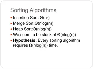
2. A General Lower Bound for Sorting We have proved that simple sorting (comparison between adjacent items) requires ?2 operations to sort N items. What about the general comparison-based sorting? We will prove that any comparison based sorting algorithm requires (?log?) comparisons. 2

3. A General Lower Bound for Sorting Consider sorting 3 numbers: a, b, and c (let us assume they are not equal). How many comparisons do we need to sort these three numbers? Can we do it with one comparison? Can we do it with two comparisons? 3

4. A General Lower Bound for Sorting Consider trying to sort 3 numbers: a, b, and c (let us assume they are not equal). How many comparisons do we need to sort these three numbers? How to model the whole process so that we do not miss any cases? What are the possible sorted orders of a, b, and c? 3 * 2 *1 cases a < b < c a < c < b b < a < c c < a < b b < c < a c < b < a At the end of any sorting algorithm, the sorting algorithm needs to come to one of these results 4

5. Modeling comparison based sorting a < b < c, a < c < b b < a < c, b < c < a c < a < b, c < b < a At the beginning, all are possibility Refine the possibilities by Comparison (eg. compare a to b) a < b b < a a < b < c, a < c < b c < a < b b < a < c, b < c < a c < b < a b < c c < b c < b b < c a < b < c a < c < b b < a < c c < a < b b < c < a c < b < a A sorting algorithm decides which two items to compare at each step. 5

6. A decision tree for three elements sort 6

7. A General Lower Bound for Sorting Back to this question: Consider sorting 3 numbers: a, b, and c (let us assume they are not equal). How many comparisons do we need to sort these three numbers? There are many such trees for sorting 3 numbers. Is there a sorting algorithm that can get the solution in 2 comparisons? The model is a binary tree with 6 leaves! The tree height is at least 3! Same idea is applied to find the lower bound for any sorting of N items. 7

8. A General Lower Bound for Sorting Decision tree: Each node in the decision tree represents a set of possible orderings of the elements consistent with the comparisons that have been made. The results of the comparisons are the tree edges. The root represents the set of all possible orderings: when the sorting algorithm is given an array to sort, any possible ordering is a possibility! Each node performs one comparison, which partitions its set of orderings into two sets based on the comparison results. The two sets are in each of its children, respectively. The algorithm needs to perform enough comparison to get to a set that contains one ordering (the sorting result). 8

9. A General lower bound for comparison based sorting Each comparison based sorting algorithm can be represented by a binary decision tree Different algorithms differ in the items selected for comparison at each node. The worst case complexity of a sorting algorithm is the largest number comparisons needed. With the decision tree model, what is the tree terminology for this? 9

10. A General lower bound for comparison based sorting Each comparison based sorting algorithm can be represented by a binary decision tree Different algorithms differ in the items selected for comparison at each node. The worst case complexity of a sorting algorithm is the largest number comparisons needed. With the decision tree model, what is the tree terminology for this? The height of the decision tree! The most efficient sorting algorithm is the one with the smallest height! The lower bound for any comparison based sorting is the height of that smallest tree. Can we figure this out? 10

11. A General lower bound for comparison based sorting The lower bound for any comparison based sorting is the height of the decision tree for the most efficient sorting algorithm. Can we figure this out? We cannot by looking at different sorting algorithms Instead, we need to look at the decision tree in general Remember how we derive a lower bound for sorting 3 numders? But do have some information about the decision tree, which allows us to derive the lower bound of the height of decision trees. What do we have? 11

12. A General lower bound for comparison based sorting But do have some information about the decision tree, what do we have about the decision tree? It is a binary tree! We know the number of leaves in the tree. The number of possible sorted orders of N items, let us denote it as X (we will figure this out later) What is shortest binary tree that can have X leaves (this is the lower bound of any binary tree) ? Complete binary tree: 2?= ? ? = lg ? 12

13. A General lower bound for comparison based sorting To get the minimum tree height of the decision tree, let us decide the number of leaves in the tree. Number of leaves = number of orderings of N numbers N! = N * (N-1) * (N-2) * * 2 * 1 For a binary tree to have N! leaves, the tree height is at least ??? ?! = log ? + log ? 1 + + 1 ? 2 log ? + log ? 1 + + log ? 2 ? 2 ? 2 log + log + + log =? ? 2 2 log = (???? ? ) No comparison based sorting algorithm can be better than O(N lg(N)) 13

14. A General lower bound for comparison based sorting For sorting N numbers, the decision tree height is at least (???? ? ). The lower bound for any comparison based sorting algorithm is at least ???? ? comparison operations in the worst case. This lower bound is achieved by Heapsort, Mergesort, and Quicksort. All of these sorting algorithms have a complexity of O(???? ? ) 14

15. Heapsort Build a binary minHeap of N elements O(N) time Then perform NdeleteMinoperations log(N) time per deleteMin Total complexity O(N log N) However it requires an extra array to store results In addition to the heap To eliminate this requirement Using heap to store sorted elements Using maxHeap instead of minHeap 15

16. Example (MaxHeap) After BuildHeap After first deleteMax 16

17. Heapsort Implementation /** * Internal method for heapsort that is used in * deleteMax and buildHeap. * i is the position from which to percolate down. * n is the logical size of the binary heap. */ template <typename Comparable> void percDown( vector<Comparable> & a, int i, int n ) { int child; Comparable tmp; // Standard heapsort. template <typename Comparable> void heapsort( vector<Comparable> & a ) { // build heap for( int i = a.size( ) / 2 - 1; i >= 0; --i ) percDown( a, i, a.size( ) ); // deleteMax for( int j = a.size( ) - 1; j > 0; --j ) { std::swap( a[ 0 ], a[ j ] ); percDown( a, 0, j ); } } /* Internal method for heapsort. * i is the index of an item in the heap. * Returns the index of the left child. */ inline int leftChild( int i ) { return 2 * i + 1; } Notice that the root is at a[0] instead of a[1]. 2NlogN comparisons for( tmp = std::move( a[ i ] ); leftChild( i ) < n; i = child ) { child = leftChild( i ); if( child != n - 1 && a[ child ] < a[ child + 1 ] ) ++child; if( tmp < a[ child ] ) a[ i ] = std::move( a[ child ] ); else break; } a[ i ] = std::move( tmp ); } 17

18. Mergesort Divide the N values to be sorted into two halves Recursively sort each half using Mergesort Base case N=1 no sorting required Merge the two sorted halves into one sorted list 18

19. Merging two sorted lists Keep a counter for each list, starting at the beginning of the lists. Compare the two values indexed by the counters, output the smaller value and increment the counter. When one list is processed, output all items in the other list. Example: merging (and sorting) the following two sorted lists. 1, 13, 24, 26 2, 15, 27, 38 Compare 1 and 2 and output 1 19

20. Merging two sorted lists 1, 13, 24, 26 output: 1 2, 15, 27, 38 ---- 1, 13, 24, 26 output: 1, 2 2, 15, 27, 38 ---- 1, 13, 24, 26 output: 1, 2, 13, 2, 15, 27, 38 ---- 1, 13, 24, 26 output: 1, 2, 13, 15 2, 15, 27, 38 Compare 13 and 2 and output 2 Compare 13 and 15 and output Compare 24 and 15 and output What is the complexity of merging two sorted lists into one sorted list? 20

21. Mergesort mergeSort(a, tmpArray, begin, end) { If ( begin + 1 == end ) return; // one item sorted! int center = ( begin + end ) / 2; mergeSort( a, tmpArray, left, center ); mergeSort( a, tmpArray, center + 1, right ); merge( a, tmpArray, left, center + 1, right ); } 21

22. Mergesort example Divide the N values to be sorted into two halves Recursively sort each half using Mergesort Base case N=1 no sorting required Merge the two sorted halves into one sorted list 16 15 14 11 10 9 8 1 2 4 7 6 5 3 12 13 16 15 14 11 10 9 8 1 2 4 7 6 5 3 12 13 16 15 14 11 10 9 8 1 2 4 7 6 5 3 12 13 16 15 14 11 10 9 8 1 2 4 7 6 5 3 12 13 At this time, the algorithm merges sorted lists of one elements 15 16 11 14 9 10 1 8 2 4 6 7 3 5 12 13 22

23. Merge sort example 15 16 11 14 9 10 1 8 2 4 6 7 3 5 12 13 11 14 15 16 1 8 9 10 2 4 6 7 3 5 12 13 1 8 9 10 11 14 15 16 2 3 4 5 6 7 12 13 1 2 3 4 5 6 7 8 9 10 11 12 13 14 15 16 23

24. Mergesort Implementation // Mergesort algorithm (driver). template <typename Comparable> void mergeSort( vector<Comparable> & a ) { vector<Comparable> tmpArray( a.size( ) ); mergeSort( a, tmpArray, 0, a.size( ) - 1 ); } /** * Internal method that makes recursive calls. * a is an array of Comparable items. * tmpArray is an array to place the merged result. * left is the left-most index of the subarray. * right is the right-most index of the subarray. */ template <typename Comparable> void mergeSort( vector<Comparable> & a, vector<Comparable> & tmpArray, int left, int right ) { if( left < right ) { int center = ( left + right ) / 2; mergeSort( a, tmpArray, left, center ); mergeSort( a, tmpArray, center + 1, right ); merge( a, tmpArray, left, center + 1, right ); } } 24

25. /** * Internal method that merges two sorted halves of a subarray. * a is an array of Comparable items. * tmpArray is an array to place the merged result. * leftPos is the left-most index of the subarray. * rightPos is the index of the start of the second half. * rightEnd is the right-most index of the subarray. */ template <typename Comparable> void merge( vector<Comparable> & a, vector<Comparable> & tmpArray, int leftPos, int rightPos, int rightEnd ) { int leftEnd = rightPos - 1; int tmpPos = leftPos; int numElements = rightEnd - leftPos + 1; // Main loop while( leftPos <= leftEnd && rightPos <= rightEnd ) if( a[ leftPos ] <= a[ rightPos ] ) tmpArray[ tmpPos++ ] = std::move( a[ leftPos++ ] ); else tmpArray[ tmpPos++ ] = std::move( a[ rightPos++ ] ); while( leftPos <= leftEnd ) // Copy rest of first half tmpArray[ tmpPos++ ] = std::move( a[ leftPos++ ] ); while( rightPos <= rightEnd ) // Copy rest of right half tmpArray[ tmpPos++ ] = std::move( a[ rightPos++ ] ); // Copy tmpArray back for( int i = 0; i < numElements; ++i, --rightEnd ) a[ rightEnd ] = std::move( tmpArray[ rightEnd ] ); } 25

26. Mergesort complexity analysis Let T(N) be the complexity when size is N Merge O(N). Recurrence relation T(N) = 2T(N/2) + N T(N) = 4T(N/4) + 2N T(N) = 8T(N/8) + 3N T(N) = 2kT(N/2k) + k*N For k = logN, 2?= 2log ?= ? T(N) = NT(1) + N logN Complexity: O(NlogN) Is mergesort in place? 26

27. Quicksort Fastest known sorting algorithm in practice Caveat: not always stable sorting Can do it as a stable sort, but some partition techniques do not guarantee this. Average case complexity O(N logN ) Worst-case complexity O(N2) Rarely happens, if coded correctly Can vary in space complexity, depending on strategies chosen. 27

28. Quicksort Outline Divide and conquer approach Given array S to be sorted If size of S < 1 then done; Pick any element v in S as the pivot Partition S-{v} (remaining elements in S) into two groups S1 = {all elements in S-{v} that are smaller than v} S2 = {all elements in S-{v} that are larger than v} Return {quicksort(S1) followed by v followed by quicksort(S2) } Trick lies in handling the partitioning (step 3). Picking a good pivot Efficiently partitioning in-place 28

29. Quicksort example 81 31 57 75 43 13 0 92 65 26 Select pivot 31 57 75 81 43 13 65 26 0 92 partition 31 57 13 81 65 26 0 92 75 43 Recursive call Recursive call 0 13 26 31 43 57 75 81 92 Merge 0 13 26 31 43 57 65 75 81 92 29

30. Picking the Pivot Pivot partitions the array into two subsets. What is the idea Pivot? Example: 13 81 92 43 31 65 57 26 75 Sorted: 13 26 31 43 57 65 75 81 92 If you have all the knowledge, which value you would pick as the pivot to have the best performance? 30

31. Picking the Pivot Partition takes O(N) time. If we pick the middle of the list, the two subsets both have roughly N/2 items T(N) = 2 T(N/2) + N, T(N) = O(N log N) same as the merge sort If we pick the side (largest or smallest) T(N) = T(N-1) + N, same as insertion sort, T(N) = O(??)? 31

32. Picking the Pivot Example: 13 81 92 43 31 65 57 26 75 Sorted: 13 26 31 43 57 65 75 81 92 Which value is the best pivot selection? Which value is the worst pivot selection? 32

33. Picking the Pivot How would you pick one? Strategy 1: Pick the first element in S Works only if input is random What if input S is sorted, or even mostly sorted? All the remaining elements would go into either S1 or S2! Terrible performance! Why worry about sorted input? Remember Quicksort is recursive, so sub-problems could be sorted Plus mostly sorted input is quite frequent 33

34. Picking the Pivot (contd.) Strategy 2: Pick the pivot randomly Would usually work well, even for mostly sorted input Unless the random number generator is not quite random! Plus random number generation is an expensive operation 34

35. Picking the Pivot (contd.) Strategy 3: Median-of-three Partitioning Ideally, the pivot should be the median of input array S Median = element in the middle of the sorted sequence Would divide the input into two almost equal partitions Unfortunately, its hard to calculate median quickly, without sorting first! So find the approximate median Pivot = median of the left-most, right-most and center element of the array S Solves the problem of sorted input 35

36. Picking the Pivot (contd.) Example: Median-of-three Partitioning Let input S = {6, 1, 4, 9, 0, 3, 5, 2, 7, 8} left=0 and S[left] = 6 right=9 and S[right] = 8 center = (left+right)/2 = 4 and S[center] = 0 Pivot = Median of S[left], S[right], and S[center] = median of 6, 8, and 0 = S[left] = 6 36

37. Partitioning Algorithm Original input : S = {6, 1, 4, 9, 0, 3, 5, 2, 7, 8} Get the pivot out of the way by swapping it with the last element 8 1 4 9 0 3 5 2 7 6 pivot Have two iterators i and j i starts at first element and moves forward j starts at last element and moves backwards 8 1 4 9 0 3 5 2 7 6 i j pivot 37

38. Partitioning Algorithm (contd.) While (i < j) Move i to the right till we find a number greater than pivot Move j to the left till we find a number smaller than pivot If (i < j)swap(S[i], S[j]) (The effect is to push larger elements to the right and smaller elements to the left) 4. Swap the pivot with S[i] 38

39. Partitioning Algorithm Illustrated i j pivot 8 1 4 9 0 3 5 2 7 6 i j Move pivot 8 1 4 9 0 3 5 2 7 6 i j pivot swap 2 1 4 9 0 3 5 8 7 6 i j pivot move 2 1 4 9 0 3 5 8 7 6 i j pivot swap 2 1 4 5 0 3 9 8 7 6 j i pivot i and j have crossed move 2 1 4 5 0 3 9 8 7 6 2 1 4 5 0 3 6 8 7 9 Swap S[i] with pivot j i pivot 39

40. Dealing with small arrays For small arrays (say, N 20), Insertion sort is faster than quicksort Quicksort is recursive So it can spend a lot of time sorting small arrays Hybrid algorithm: Switch to using insertion sort when problem size is small (say for N < 20) 40

41. Quicksort Driver Routine /** * Quicksort algorithm (driver). */ template <typename Comparable> void quicksort( vector<Comparable> & a ) { quicksort( a, 0, a.size( ) - 1 ); } 41

42. Quicksort Pivot Selection Routine /** * Return median of left, center, and right. * Order these and hide the pivot. */ template <typename Comparable> const Comparable & median3( vector<Comparable> & a, int left, int right ) { int center = ( left + right ) / 2; Swap a[left], a[center] and a[right] in-place if( a[ center ] < a[ left ] ) std::swap( a[ left ], a[ center ] ); if( a[ right ] < a[ left ] ) std::swap( a[ left ], a[ right ] ); if( a[ right ] < a[ center ] ) std::swap( a[ center ], a[ right ] ); Pivot is in a[center] now // Place pivot at position right - 1 std::swap( a[ center ], a[ right - 1 ] ); return a[ right - 1 ]; } Swap the pivot a[center] with a[right-1] 42

43. Quicksort routine /*a is an array of Comparable items. * left is the left-most index of the subarray. right is the right-most index of the subarray. */ template <typename Comparable> void quicksort( vector<Comparable> & a, int left, int right ) { if( left + 10 <= right ) { const Comparable & pivot = median3( a, left, right ); // has a side effect // Begin partitioning int i = left, j = right - 1; for( ; ; ) { while( a[ ++i ] < pivot ) { } while( pivot < a[ --j ] ) { } if( i < j ) std::swap( a[ i ], a[ j ] ); else break; } std::swap( a[ i ], a[ right - 1 ] ); // Restore pivot quicksort( a, left, i - 1 ); // Sort small elements quicksort( a, i + 1, right ); // Sort large elements } else // Do an insertion sort on the subarray insertionSort( a, left, right ); } move swap 43

44. Runtime analysis Worst-case Average case Best case 44

45. Reading Assignment Chapter 7.11 Linear time sorts: Bucket Sort and Radix sort! 45