Explore the concepts of independence and the multiplication rule in probability theory. Learn how to calculate the probability of events using these rules with practical examples, such as determining the likelihood of selecting individuals with a specific blood type. Enhance your knowledge of probability to make informed statistical inferences.
Please find below an Image/Link to download the presentation.
The content on the website is provided AS IS for your information and personal use only. It may not be sold, licensed, or shared on other websites without obtaining consent from the author. If you encounter any issues during the download, it is possible that the publisher has removed the file from their server.
You are allowed to download the files provided on this website for personal or commercial use, subject to the condition that they are used lawfully. All files are the property of their respective owners.
The content on the website is provided AS IS for your information and personal use only. It may not be sold, licensed, or shared on other websites without obtaining consent from the author.
12.0 General Rules of Probability Connecting Chapter 12 to our Current Knowledge of Statistics Probability theory leads us from data collection to inference. The introduction to probability from Chapter 10 will now be fortified by additional rules to allow us to consider multiple types of events. The rules of probability will help us develop models so that we can generalize from our (properly collected) sample to our population of interest.
12.1 Independence and the Multiplication Rule Independence Two events A and B are independent if knowing that one occurs does not change the probability that the other occurs. Thus, if A and B are independent, P(A and B) = P(A)*P(B)
12.1 Independence and the Multiplication Rule Example: Blood Types Someone with type O-negative blood is considered to be a universal donor. According to the American Association of Blood Banks, 39% of people are type O-negative. Two unrelated people are selected at random. Calculate the probability that both have type O-negative blood.
12.1 Independence and the Multiplication Rule Example: Blood Types Someone with type O-negative blood is considered to be a universal donor. According to the American Association of Blood Banks, 39% of people are type O-negative. Two unrelated people are selected at random. Calculate the probability that both have type O-negative blood. We can apply the concept of independence. P(both type O-negative) = P(first type O-) P(second type O-negative)
12.1 Independence and the Multiplication Rule Example: Blood Types Someone with type O-negative blood is considered to be a universal donor. According to the American Association of Blood Banks, 39% of people are type O-negative. Two unrelated people are selected at random. Calculate the probability that both have type O-negative blood. We can apply the concept of independence. P(both type O-negative) = P(first type O-) P(second type O-negative) = (0.39)(0.39) (Independence)
12.1 Independence and the Multiplication Rule Example: Blood Types Someone with type O-negative blood is considered to be a universal donor. According to the American Association of Blood Banks, 39% of people are type O-negative. Two unrelated people are selected at random. Calculate the probability that both have type O-negative blood. We can apply the concept of independence. P(both type O-negative) = P(first type O-) P(second type O-negative) = (0.39)(0.39) (Independence) = 0.1521
12.1 Independence and the Multiplication Rule Example/Poll: Blood Types Suppose two unrelated people are selected at random. Calculate the probability that neither have type O-negative blood.
12.1 Independence and the Multiplication Rule Example/Poll: Blood Types Suppose two unrelated people are selected at random. Calculate the probability that neither have type O-negative blood. We can again apply the concept of independence. P(neither type is O-) = P(not O-) P(not O-) = (0.61)(0.61) (Independence) = 0.3721
12.2 The General Addition Rule The General Addition Rule Two-Way tables are helpful ways to picture two events. Venn diagrams are an alternative means of displaying multiple events. Both can be used to answer many questions involving probabilities.
12.2 The General Addition Rule Venn Diagrams and Probabilities Example: In a sample of 1000 people, 88.7% of them were right-hand dominant, 47.5% of them were female, and 42.5% of them were female and right-hand dominant. Draw a Venn diagram for this situation. .887 = .462 + .425 P(R) =P(M and R) + P(F and R) .475 = .425 + .050 P(F) = P(F and R) + P(F and L) 0.462 0.425 0.050 0.063
12.2 The General Addition Rule Venn Diagrams and Probabilities .887 = .462 + .425 P(R) =P(M and R) + P(F and R) .475 = .425 + .050 P(F) = P(F and R) + P(F and L) 0.462 0.425 0.050 0.063 Calculate the probability that a randomly selected person is right-hand dominant or female.
12.2 The General Addition Rule Venn Diagrams and Probabilities .887 = .462 + .425 P(R) =P(M and R) + P(F and R) .475 = .425 + .050 P(F) = P(F and R) + P(F and L) 0.462 0.425 0.050 0.063 Calculate the probability that a randomly selected person is right-hand dominant or female. 1st Method 0.462 + 0.425 + 0.050 = 0.937
12.2 The General Addition Rule Venn Diagrams and Probabilities .887 = .462 + .425 P(R) =P(M and R) + P(F and R) .475 = .425 + .050 P(F) = P(F and R) + P(F and L) 0.462 0.425 0.050 0.063 Calculate the probability that a randomly selected person is right-hand dominant or female. 1st Method 0.462 + 0.425 + 0.050 = 0.937 Let R = right-hand dominant (.887), and let F = female (.475).
12.2 The General Addition Rule Venn Diagrams and Probabilities .887 = .462 + .425 P(R) =P(M and R) + P(F and R) .475 = .425 + .050 P(F) = P(F and R) + P(F and L) 0.462 0.425 0.050 0.063 Calculate the probability that a randomly selected person is right-hand dominant or female. 1st Method 0.462 + 0.425 + 0.050 = 0.937 Let R = right-hand dominant (.887), and let F = female (.475). 2nd Method This is actually = P(R) + P(F) P(R and F) = P(R or F) 0.887 + 0.475 0.425 = 0.937
12.2 The General Addition Rule The General Addition Rule We just used the general addition rule: For any two events A and B, P(A or B) = P(A) + P(B) P(A and B). Question: Where did we see this concept previously?
12.2 The General Addition Rule The General Addition Rule We just used the general addition rule: For any two events A and B, P(A or B) = P(A) + P(B) P(A and B). Question: Where did we see this concept previously? OR questions from Chapter 6 where two events overlapped.
12.2 The General Addition Rule The Addition Rule for Disjoint Events What if there is no overlap of the events A and B? Events A and B are disjoint if they have no outcomes in common. Question: What is P(A or B) when A and B are disjoint?
12.2 The General Addition Rule The Addition Rule for Disjoint Events What if there is no overlap of the events A and B? Events A and B are disjoint if they have no outcomes in common. Question: What is P(A or B) when A and B are disjoint? P(A and B) = 0 (no outcomes in common)
12.2 The General Addition Rule The Addition Rule for Disjoint Events What if there is no overlap of the events A and B? Events A and B are disjoint if they have no outcomes in common. Question: What is P(A or B) when A and B are disjoint? P(A and B) = 0 (no outcomes in common) P(A or B) = P(A) + P(B) P(A and B) (General Addition Rule)
12.2 The General Addition Rule The Addition Rule for Disjoint Events What if there is no overlap of the events A and B? Events A and B are disjoint if they have no outcomes in common. Question: What is P(A or B) when A and B are disjoint? P(A and B) = 0 (no outcomes in common) P(A or B) = P(A) + P(B) P(A and B) (General Addition Rule) = P(A) + P(B) 0 (Disjoint)
12.2 The General Addition Rule The Addition Rule for Disjoint Events What if there is no overlap of the events A and B? Events A and B are disjoint if they have no outcomes in common. Question: What is P(A or B) when A and B are disjoint? P(A and B) = 0 (no outcomes in common) P(A or B) = P(A) + P(B) P(A and B) (General Addition Rule) = P(A) + P(B) 0 (Disjoint) P(A or B) = P(A) + P(B)
12.2 The General Addition Rule The Complement Rule and Addition Rule 0.462 0.425 0.050 0.063 Calculate the probability that a randomly selected person is neither right-hand dominant nor female.
12.2 The General Addition Rule The Complement Rule and Addition Rule 0.462 0.425 0.050 0.063 Calculate the probability that a randomly selected person is neither right-hand dominant nor female. P(neither R nor F) = 1 P(R or F)
12.2 The General Addition Rule The Complement Rule and Addition Rule 0.462 0.425 0.050 0.063 Calculate the probability that a randomly selected person is neither right-hand dominant nor female. P(neither R nor F) = 1 P(R or F) = 1 0.937 = 0.063
12.2 The General Addition Rule The Complement Rule and Addition Rule 0.462 0.425 0.050 0.063 Calculate the probability that a randomly selected person is neither right-hand dominant nor female. P(neither R nor F) = 1 P(R or F) = 1 0.937 = 0.063 We just used the complement rule: For any event A, P(A does not occur) = P(not A) = 1 P(A).
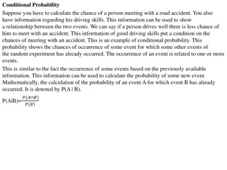
12.3 Conditional Probability Conditional Probability When P(A) > 0, the conditional probability of B given A is ? ? ? =?(? ??? ?) ?(?) Note that since P(B|A) assumes that the event A has occurred, P(A) will be greater than 0.
12.3 Conditional Probability Conditional Probability Note: Wording for conditional probabilities can often be subtle, so be sure to read carefully. Occasionally you will come across problems that embed conditional probabilities into the question. Consider the following example: Example: Calculate the probability that a randomly selected female is right-hand dominant. ? ? ? = ?(? ??? ?) ?(?)
12.3 Conditional Probability Conditional Probability Note: Wording for conditional probabilities can often be subtle, so be sure to read carefully. Occasionally you will come across problems that embed conditional probabilities into the question. Consider the following example: Example: Calculate the probability that a randomly selected female is right-hand dominant. ? ? ? = ?(? ??? ?) = .??? .??? ?(?)
12.3 Conditional Probability Conditional Probability Note: Wording for conditional probabilities can often be subtle, so be sure to read carefully. Occasionally you will come across problems that embed conditional probabilities into the question. Consider the following example: Example: Calculate the probability that a randomly selected female is right-hand dominant. ? ? ? = ?(? ??? ?) = .??? .??? = 0.8947 ?(?)
12.3 Conditional Probability Conditional Probability The | means given. The event behind the | is the conditioning event. The idea of a conditional probability P(B|A) of one event B given that another event A occurs is the proportion of all occurrences of A for which B also occurs.
12.4 General Multiplication Rule General Multiplication Rule The probability that both of two events A and B happen together can be found by ? ? ??? ? = ? ? ?(?|?) Here P(B|A) is the conditional probability that B occurs given the information that A occurs.
12.4 General Multiplication Rule Example: Internet Access An A.C. Nielsen study found that 81% of households in the United States have computers. Of those 81%, 92% have Internet access. Calculate the probability that a randomly selected U.S. household has a computer and has Internet access.
12.4 General Multiplication Rule Example: Internet Access An A.C. Nielsen study found that 81% of households in the United States have computers. Of those 81%, 92% have Internet access. Calculate the probability that a randomly selected U.S. household has a computer and has Internet access. Let C =household has a computer. Let I = household has Internet access.
12.4 General Multiplication Rule Example: Internet Access An A.C. Nielsen study found that 81% of households in the United States have computers. Of those 81%, 92% have Internet access. Calculate the probability that a randomly selected U.S. household has a computer and has Internet access. Let C =household has a computer. Let I = household has Internet access. P(C and I)
12.4 General Multiplication Rule Example: Internet Access An A.C. Nielsen study found that 81% of households in the United States have computers. Of those 81%, 92% have Internet access. Calculate the probability that a randomly selected U.S. household has a computer and has Internet access. Let C =household has a computer. Let I = household has Internet access. P(C and I) = P(C) P(I|C)
12.4 General Multiplication Rule Example: Internet Access An A.C. Nielsen study found that 81% of households in the United States have computers. Of those 81%, 92% have Internet access. Calculate the probability that a randomly selected U.S. household has a computer and has Internet access. Let C =household has a computer. Let I = household has Internet access. P(C and I) = P(C) P(I|C) = (0.81)(0.92) = 0.7452
10.2 Randomness and Probability Poll Two unrelated persons are in line to donate blood. The blood type of the 2nd person is not impacted by the blood type of the first. a) True b) False
10.2 Randomness and Probability Poll Two unrelated persons are in line to donate blood. The blood type of the 2nd person is not impacted by the blood type of the first. a) True b) False
12.5 Independence Again Definition: Independence Two events A and B that both have positive probability are independent if ? ? ? = ?(?) The fact that A has occurred does not impact B s probability of occurrence.
12.5 Independence Again Let Sz= Zachary s decision to smoke. Let SM = Megan s decision to smoke. Example: Smoking Smoking has been a hot topic in recent months. Twenty percent of people (in a city with a population in of about 1 million) are smokers. Two people, Megan and Zach, are selected at random. Confirm mathematically and practically, that Megan s decision to smoke is independent of Zach s.
12.5 Independence Again Let Sz= Zachary s decision to smoke. Let SM = Megan s decision to smoke. Example: Smoking Smoking has been a hot topic in recent months. Twenty percent of people (in a city with a population in of about 1 million) are smokers. Two people, Megan and Zach, are selected at random. Confirm mathematically and practically, that Megan s decision to smoke is independent of Zach s. Mathematically, P(SM and SZ )
12.5 Independence Again Let Sz= Zachary s decision to smoke. Let SM = Megan s decision to smoke. Example: Smoking Smoking has been a hot topic in recent months. Twenty percent of people (in a city with a population in of about 1 million) are smokers. Two people, Megan and Zach, are selected at random. Confirm mathematically and practically, that Megan s decision to smoke is independent of Zach s. Mathematically, P(SM and SZ ) =P(SM )*P(SZ |SM) gen.rule of mult.
12.5 Independence Again Let Sz= Zachary s decision to smoke. Let SM = Megan s decision to smoke. Example: Smoking Smoking has been a hot topic in recent months. Twenty percent of people (in a city with a population in of about 1 million) are smokers. Two people, Megan and Zach, are selected at random. Confirm mathematically and practically, that Megan s decision to smoke is independent of Zach s. Mathematically, P(SM and SZ ) =P(SM )*P(SZ |SM) gen.rule of mult. =200,000 1,000,000 199,999 999,999
12.5 Independence Again Let Sz= Zachary s decision to smoke. Let SM = Megan s decision to smoke. Example: Smoking Smoking has been a hot topic in recent months. Twenty percent of people (in a city with a population in of about 1 million) are smokers. Two people, Megan and Zach, are selected at random. Confirm mathematically and practically, that Megan s decision to smoke is independent of Zach s. Mathematically, P(SM and SZ ) =P(SM )*P(SZ |SM) gen.rule of mult. 999,999=39999800000 99999999999 =200,000 1,000,000 199,999
12.5 Independence Again Let Sz= Zachary s decision to smoke. Let SM = Megan s decision to smoke. Example: Smoking Smoking has been a hot topic in recent months. Twenty percent of people (in a city with a population in of about 1 million) are smokers. Two people, Megan and Zach, are selected at random. Confirm mathematically and practically, that Megan s decision to smoke is independent of Zach s. Mathematically, P(SM and SZ ) =P(SM )*P(SZ |SM) gen.rule of mult. P(SM and SZ ) = .03999984 = 4 ??? ??????? ? 999,999=39999800000 99999999999 =200,000 1,000,000 199,999
12.5 Independence Again Let Sz= Zachary s decision to smoke. Let SM = Megan s decision to smoke. Example: Smoking Smoking has been a hot topic in recent months. Twenty percent of people (in a city with a population in of about 1 million) are smokers. Two people, Megan and Zach, are selected at random. Confirm mathematically and practically, that Megan s decision to smoke is independent of Zach s. Mathematically, P(SM and SZ ) =P(SM )*P(SZ |SM) gen.rule of mult. P(SM and SZ ) = .03999984 = 4 ??? ??????? ? P(SM and SZ ) =.04 999,999=39999800000 99999999999 =200,000 1,000,000 199,999
12.5 Independence Again Let Sz= Zachary s decision to smoke. Let SM = Megan s decision to smoke. Example: Smoking Smoking has been a hot topic in recent months. Twenty percent of people (in a city with a population in of about 1 million) are smokers. Two people, Megan and Zach, are selected at random. Confirm mathematically and practically, that Megan s decision to smoke is independent of Zach s. Mathematically, P(SM and SZ ) =P(SM )*P(SZ |SM) gen.rule of mult. P(SM and SZ ) = .03999984 = 4 ??? ??????? ? P(SM and SZ ) =.04 = .20*.20 999,999=39999800000 99999999999 =200,000 1,000,000 199,999
12.5 Independence Again Let Sz= Zachary s decision to smoke. Let SM = Megan s decision to smoke. Example: Smoking Smoking has been a hot topic in recent months. Twenty percent of people (in a city with a population in of about 1 million) are smokers. Two people, Megan and Zach, are selected at random. Confirm mathematically and practically, that Megan s decision to smoke is independent of Zach s. Mathematically, P(SM and SZ ) =P(SM )*P(SZ |SM) gen.rule of mult. P(SM and SZ ) = .03999984 = 4 ??? ??????? ? P(SM and SZ ) =.04 = .20*.20 = P(SM )*P(SZ) (independence) 999,999=39999800000 99999999999 =200,000 1,000,000 199,999
12.5 Independence Again Let Sz= Zachary s decision to smoke. Let SM = Megan s decision to smoke. Example: Smoking Smoking has been a hot topic in recent months. Twenty percent of people (in a city with a population in of about 1 million) are smokers. Two people, Megan and Zach, are selected at random. Confirm mathematically and practically, that Megan s decision to smoke is independent of Zach s. Mathematically, P(SM and SZ ) =P(SM )*P(SZ |SM) gen.rule of mult. P(SM and SZ ) = .03999984 = 4 ??? ??????? ? P(SM and SZ ) =.04 = .20*.20 = P(SM )*P(SZ) (independence) 999,999=39999800000 99999999999 =200,000 1,000,000 199,999 Practically, Zach s decision to smoke is not influenced by a randomly selected person from the same city (Megan, in this case).