Generating Random Deviates from Various Distributions

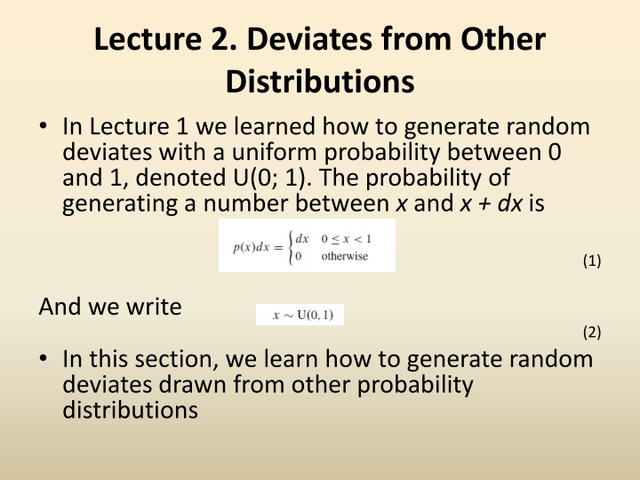
Lecture 2. Deviates from Other Distributions In Lecture 1 we learned how to generate random deviates with a uniform probability between 0 and 1, denoted U(0; 1). The probability of generating a number between x and x + dx is (1) And we write (2) In this section, we learn how to generate random deviates drawn from other probability distributions

Exponential Deviates Suppose that we generate a uniform deviate x and then take some prescribed function of it, y(x). The probability distribution of y, denoted p(y)dy, is determined by the fundamental transformation law of probabilities, which is simply (3) (4) As an example, take (5) with x ~ U(0; 1). Then (6) which is the exponential distribution with unit mean.

This distribution occurs frequently in real life, usually as the distribution of waiting times between independent Poisson-random events, for example the radioactive decay of nuclei. You can also easily see (from 6) that the quantity y/ has the probability distribution e- y, so (7) We can thus generate exponential deviates at a cost of about one uniform deviate, plus a logarithm, per call.

Transformation Method in General Let s see what is involved in using the above transformation method to generate some arbitrary desired distribution of y s, say one with p(y) = f(y) for some positive function f whose integral is 1. According to (4), we need to solve the differential equation (8) But the solution of this is just x = F(y), where F(y) is the indefinite integral of f(y). The desired transformation that takes a uniform deviate into one distributed as f(y) is therefore (9) where F-1is the inverse function to F . Whether (9) is feasible to implement depends on whether the inverse function of the integral of f(y) is itself feasible to compute, either analytically or numerically. Sometimes it is, and sometimes it isn t. Incidentally, (9) has an immediate geometric interpretation: Since F(y) is the area under the probability curve to the left of y, (9) is just the prescription: Choose a uniform random x, then find the value y that has that fraction x of probability area to its left, and return the value y.

Normal Deviates by Transformation (Box-Muller) Transformation methods generalize to more than one dimension. If x1, x2, are random deviates with a joint probability distribution p(x1; x2; )dx1dx2 , and if y1; y2; are each functions of all the x s (same number of y s as x s), then the joint probability distribution of the y s is (10) An important historical example of the use of (10) is the Box-Muller method for generating random deviates with a normal (Gaussian) distribution (11) Consider the transformation between two uniform deviates on (0,1), x1; x2, and two quantities y1; y2, (12)

Equivalently we can write (13) Now the Jacobian determinant can readily be calculated (14) Since this is the product of a function of y2alone and a function of y1alone, we see that each y is independently distributed according to the normal distribution (11). One further trick is useful in applying (12). Suppose that, instead of picking uniform deviates x1and x2in the unit square, we instead pick v1and v2as the ordinate and abscissa of a random point inside the unit circle around the origin. Then the sum of their squares, R2 = v12 + v22, is a uniform deviate, which can be used for x1, while the angle that (v1; v2) defines with respect to the v1-axis can serve as the random angle 2 x2.

Rayleigh Deviates The Rayleigh distribution is defined for positive z by (15) Since the indefinite integral can be done analytically, and the result easily inverted, a simple transformation method from a uniform deviate x results: (16) A Rayleigh deviate z can also be generated from two normal deviates y1and y2by (17) Indeed, the relation between equations (16) and (17) is immediately evident in the equation for the Box-Muller method, equation (12), if we square and sum that method s two normal deviates y1and y2.

Rejection Method The rejection method is a powerful, general technique for generating random deviates whose distribution function p(x)dx (probability of a value occurring between x and x + dx) is known and computable. The rejection method does not require that the cumulative distribution function (indefinite integral of p(x)) be readily computable, much less the inverse of that function which was required for the transformation method in the previous section. The rejection method is based on a simple geometrical argument:

Draw a graph of the probability distribution p(x) that you wish to generate, so that the area under the curve in any range of x corresponds to the desired probability of generating an x in that range. If we had some way of choosing a random point in two dimensions, with uniform probability in the area under your curve, then the x value of that random point would have the desired distribution. Now, on the same graph, draw any other curve f(x) that has finite (not infinite) area and lies everywhere above your original probability distribution. We will call this f(x) the comparison function. Imagine now that you have some way of choosing a random point in two dimensions that is uniform in the area under the comparison function. Whenever that point lies outside the area under the original probability distribution, we will reject it and choose another random point. Whenever it lies inside the area under the original probability distribution, we will accept it.

Cauchy Deviates The defining probability density is The cdf is given by The inverse cdf is given by The further trick described following equation (14) in the context of the Box-Muller method is now seen to be a rejection method for getting trigonometric functions of a uniformly random angle. If we combine this with the explicit formula for the inverse cdf of the Cauchy distribution, we can generate Cauchy deviates quite efficiently.

Ratio-of-Uniforms Method In finding Cauchy deviates, we took the ratio of two uniform deviates chosen to lie within the unit circle. If we generalize to shapes other than the unit circle, and combine it with the principle of the rejection method, a powerful variant emerges. Deviates of virtually any probability distribution p(x) can be generated by the following rather amazing prescription: Construct the region in the (u; v) plane bounded by 0 <= u <= [p(v/u)]1/2 Choose two deviates, u and v, that lie uniformly in this region. Return v/u as the deviate.

Proof: We can represent the ordinary rejection method by the equation in the (x; p) plane, (18) Since the integrand is 1, we are justified in sampling uniformly in (x; p ) as long as p is within the limits of the integral (that is, 0 < p < p(x)). Now make the change of variable (19) Then equation (18) becomes (20)

Typically this ratio-of-uniforms method is used when the desired region can be closely bounded by a rectangle, parallelogram, or some other shape that is easy to sample uniformly. Then, we go from sampling the easy shape to sampling the desired region by rejection of points outside the desired region. An important adjunct to the ratio-of-uniforms method is the idea of a squeeze. A squeeze is any easy-to-compute shape that tightly bounds the region of acceptance of a rejection method, either from the inside or from the outside. Best of all is when you have squeezes on both sides. Then you can immediately reject points that are outside the outer squeeze and immediately accept points that are inside the inner squeeze. Squeezes are useful both in the ordinary rejection method and in the ratio-of-uniforms method.

Normal Deviates by Ratio-of- Uniforms

Gamma Deviates If is a small positive integer, a fast way to generate x ~ Gamma( , ) is to use the fact that it is distributed as the waiting time to the -th event in a Poisson random process of unit mean. Since the time between two consecutive events is just the exponential distribution Exponential(1), you can simply add up exponentially distributed waiting times, i.e., logarithms of uniform deviates. Even better, since the sum of logarithms is the logarithm of the product, you really only have to compute the product of a uniform deviates and then take the log. When < 1, the gamma distribution s density function is not bounded, which is inconvenient. However, it turns out that if (22) then (23)

For > 1, we use rejection method based on a simple transformation of the gamma distribution combined with a squeeze. After transformation, the gamma distribution can be bounded by a Gaussian curve whose area is never more than 5% greater than that of the gamma curve. The cost of a gamma deviate is thus only a little more than the cost of the normal deviate that is used to sample the comparison function.

Distributions Easily Generated by Other Deviates From normal, gamma and uniform deviates, we get a bunch of other distributions for free. Important: When you are going to combine their results, be sure that all distinct instances of Normaldist, Gammadist, and Ran have different random seeds! Chi-Square Deviates

Student-t Deviates Deviates from the Student-t distribution can be generated by a method very similar to the Box-Muller method. The analog of equation (12) is If u1 and u2 are independently uniform, U(0; 1), then or Unfortunately, you can t do the Box-Muller trick of getting two deviates at a time, because the Jacobian determinant analogous to equation (14) does not factorize. You might want to use the polar method anyway, just to get cos 2 u2, but its advantage is now not so large. An alternative method uses the quotients of normal and gamma deviates. If we have then

Beta Deviates If then F-Distribution Deviates If then

Poisson Deviates The Poisson distribution, Poisson( ), is a discrete distribution, so its deviates will be integers, k. To use the methods already discussed, it is convenient to convert the Poisson distribution into a continuous distribution by the following trick: Consider the finite probability p(k) as being spread out uniformly into the interval from k to k+1. This defines a continuous distribution q (k)dk given by (36) If we now use a rejection method, or any other method, to generate a (noninteger) deviate from (36), and then take the integer part of that deviate, it will be as if drawn from the discrete Poisson distribution (See Figure 7.3.4.) This trick is general for any integer-valued probability distribution. Instead of the floor operator, one can equally well use ceiling or nearest anything that spreads the probability over a unit interval.

For large enough, the distribution (36) is qualitatively bell-shaped (albeit with a bell made out of small, square steps). In that case, the ratio-of-uniforms method works well. It is not hard to find simple inner and outer squeezes in the (u; v) plane of the form v2 = Q(u), where Q(u) is a simple polynomial in u. The only trick is to allow a big enough gap between the squeezes to enclose the true, jagged, boundaries for all values of . (Look ahead to Figure 7.3.5 for a similar example.) For intermediate values of , the jaggedness is so large as to render squeezes impractical, but the ratio- of-uniforms method, unadorned, still works pretty well. For small , we can use an idea similar to that mentioned above for the gamma distribution in the case of integer a. When the sum of independent exponential deviates first exceeds , their number (less 1) is a Poisson deviate k. Also, as explained for the gamma distribution, we can multiply uniform deviates from U(0; 1) instead of adding deviates from Exponential(1).

Binomial Deviates The generation of binomial deviates k ~ Binomial(n; p) involves many of the same ideas as for Poisson deviates. The distribution is again integer- valued, so we use the same trick to convert it into a stepped continuous distribution. We can always restrict attention to the case p <= 0.5, since the distribution s symmetries let us trivially recover the case p > 0.5. When n > 64 and np > 30, we use the ratio-of-uniforms method, with squeezes shown in Figure 7.3.5. It would be foolish to waste much thought on the case where n > 64 and np < 30, because it is so easy simply to tabulate the cdf, say for 0 k < 64, and then loop over k s until the right one is found. (A bisection search, implemented below, is even better.) With a cdf table of length 64, the neglected probability at the end of the table is never larger than ~10-20. (At 109 deviates per second, you could run 3000 years before losing a deviate.) What is left is the interesting case n < 64, which we will explore in some detail, because it demonstrates the important concept of bit-parallel random comparison.

Analogous to the methods for gamma deviates with small integer a and for Poisson deviates with small , is this direct method for binomial deviates: Generate n uniform deviates in U(0; 1). Count the number of them < p. Return the count as k ~ Binomial(n; p). Indeed this is essentially the definition of a binomial process! The problem with the direct method is that it seems to require n uniform deviates, even when the mean value of k is much smaller. Would you be surprised if we told you that for n <= 64 you can achieve the same goal with at most seven 64-bit uniform deviates, on average? Here is how. Expand p < 1 into its first 5 bits, plus a residual, (37) where each bi is 0 or 1, and 0 <= pr <= 1. Now imagine that you have generated and stored 64 uniform U(0; 1) deviates, and that the 64-bit word P displays just the first bit of each of the 64. Compare each bit of P to b1. If the bits are the same, then we don t yet know whether that uniform deviate is less than or greater than p. But if the bits are different, then we know that the generator is less than p (in the case that b1 = 1) or greater than p (in the case that b1= 0). If we keep a mask of known versus unknown cases, we can do these comparisons in a bit-parallel manner by bitwise logical operations (see code below to learn how). Now move on to the second bit, b2, in the same way. At each stage we change half the remaining unknowns to knowns. After five stages (for n = 64) there will be two remaining unknowns, on average, each of which we finish off by generating a new uniform and comparing it to pr .

The trick is that the bits used in the five stages are not actually the leading five bits of 64 generators, they are just five independent 64-bit random integers. The number five was chosen because it minimizes 64x2-j +j , the expected number of deviates needed.

Multivariate Normal Deviates A multivariate random deviate of dimension M is a point in M- dimensional space. Its coordinates are a vector, each of whose M components are random but not, in general, independently so, or identically distributed. The special case of multivariate normal deviates is defined by the multidimensional Gaussian density function where the parameter is a vector that is the mean of the distribution, and the parameter is a symmetrical, positive-definite matrix that is the distribution s covariance. There is a quite general way to construct a vector deviate x with a specified covariance and mean , starting with a vector y of independent random deviates of zero mean and unit variance: First, use Cholesky decomposition to factor into a left triangular matrix L times its transpose,

Next, whenever you want a new deviate x, fill y with independent deviates of unit variance and then construct