Genetic Covariance Structure Analysis in Classical Twin Design

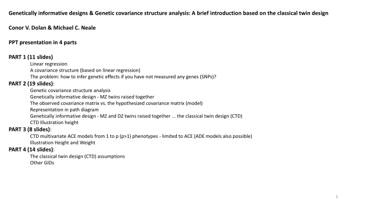
Genetically informative designs & Genetic covariance structure analysis: A brief introduction based on the classical twin design Conor V. Dolan & Michael C. Neale PPT presentation in 4 parts PART 1 (11 slides) Linear regression A covariance structure (based on linear regression) The problem: how to infer genetic effects if you have not measured any genes (SNPs)? PART 2 (19 slides): Genetic covariance structure analysis Genetically informative design - MZ twins raised together The observed covariance matrix vs. the hypothesized covariance matrix (model) Representation in path diagram Genetically informative design - MZ and DZ twins raised together ... the classical twin design (CTD) CTD Illustration height PART 3 (8 slides): CTD multivariate ACE models from 1 to p (p>1) phenotypes - limited to ACE (ADE models also possible) Illustration Height and Weight PART 4 (14 slides): The classical twin design (CTD) assumptions Other GIDs 1

Genetically informative design & Genetic covariance structure analysis: A brief introduction based on the classical twin design Conor V. Dolan & Michael C. Neale PPT presentation in 4 parts .... PART 1 (12 slides) Linear regression A covariance structure (based on linear regression) The problem: how to infer genetic effects if you have not measured any genes (SNPs)? 2

Fitting models to phenotypic data in genetically informative designs (GID) using genetic covariance structure modeling (GCSM) Aim: infer genetic and environmental contributions to phenotypic variance from the phenotypic covariances (correlations) among family members (no measured genotypes, no measured environmental variables) Contributions are expressed as variance components , so the the phenotypic variance is decomposed into variance components. Start with something familiar: the linear regression model (e.g., as used in GWAS) 3

Linear regression model: predict Y from X .... equation: Yi= b0+ b1*Xi+ ei ... e.g. GWAS: Heighti= b0+ b1*SNPi+ ei variables: Yi Xi ei b0 b1 dependent (predicted) in participant i (EA, Height, Depression) predictor in participant i (genetic variant: a SNP) residual in participant i intercept slope or regression coefficient parameters: Y, X and e are variables because their value vary over persons b0and b1are (fixed) parameters, with unknown values (in the well defined population) Are X and Y linearly related? Null hypothesis (H-null): b1=0 4

N = 20000 Descriptives height: mean = 180.03 var= 64.01 SNP: mean = 0.80 var = 0.48 Covariance matrix height 64.01 0.212 SNP 0.212 0.480 height SNP Correlation matrix height 1.000 0.038 SNP 0.038 1.000 height SNP Alleles A-a, genotypes aa, Aa/aA and AA, coded 0, 1, 2 (Note this is additive coding) 5

Results of linear regression analysis (in R). Estimate Std. Error t value Pr(>|t|) (Intercept) 179.67245 0.08635 2080.67 < 2e-16 *** SNP 0.44226 0.08160 5.42 6.02e-08 *** b0 b1 Linear association? H-null b1=0, H-alt b1 0, =0.01 Conclusion: p< (p= 6.02e-08) so we reject H-null Conclusion: individual differences in height are linearly related to Individual differences in SNP; or SNP explains variance of height or the SNP is associated with height. Linear additive model: the effect of alleles A on height is additive go from aa (0) to Aa (1) is associated with difference .44226 (b1) go from aa (0) to AA (2) is associated with difference .44226 + .44226 (additive: b1+ b1) 6

Heighti= b0+ b1*SNPi+ ei = 197.67 + .442*SNPi+ ei Increase in the number of A alleles (from aa to Aa and from Aa to AA) is associated with increase in height of b1= 0.442 cm. Because the SNP is coded 0 (aa) / 1 (Aa, aA) / 2 (AA) and the model is linear, the explained variance is called additive genetic variance. R2: 0.001467 proportion of variance explained or 0.1467% Covariance structure model: The linear regression model 1) provides an account of the covariance (correlation) of Height and SNP (remember correlation expression linear association) 2) provide a decomposition of variance of Height (remember: variance is a measure of the magnitude of individual differences) 7

covariance matrix observed numerical cov S Height in symbols Height s2H sH,SNP SNP SNP Height 64.01 0.212 Height sH,SNP s2SNP SNP 0.212 0.480 SNP based on linear regression model Height b12*s2SNP+s2e SNP b1*s2SNP SNP b1*s2SNP s2SNP Height Heighti= b0+ b1*SNPi+ ei .... Heighti= 197.67 + .442*SNPi+ ei 8

linear regression model Height b12*s2SNP +s2e b1*s2SNP Observed numerical Height Height 64.01 SNP 0.212 SNP b1*s2SNP s2SNP SNP 0.212 0.480 Height SNP s2H= b12*s2SNP +s2e = .4422*0.480 = 0.0938 (i.e. explained additive genetic variance) Decomposition: b1*s2SNP= .442*0.480 = .212 Covariance: Effect size R2: {b12*s2SNP} / { b12*s2SNP +s2e} = 0.0938 / 64.01 = .00146, or .146% 9

model: linear regression model Heighti= b0+ b1*SNPi+ ei linear regression model - implied covariance structure Height SNP model implied covariance structure b12*s2SNP +s2e 64.01 b1*s2SNP 0.212 Height b1*s2SNP 0.212 s2SNP 0.480 SNP b1 1 SNP Height e path diagram s2e s2SNP 10

an observed variable, a measured variable (phenotype, locus) Height A a latent variable, unobservable variable (additive genetic factor) neuro- ticism a latent variable, unobservable variable (the neuroticism as a latent construct) conventions neuroticism as measured using a psychometric test, a test score (the test score approximates the latent construct) neuro- ticism X Y e regression relationship - linear association (asymmetric) covariance or correlation - linear association (symmetric) Y X X variance 11

Suppose we measured all SNPs relevant to height, suppose there are just 2 Heighti= b0+ b1*SNP1i+ b2*SNP2i + ei Ai= b1*SNP1i+ b2*SNP2i s2SNP1 s2A s2E s2E b1 SNP1 1 1 1 E H A s12 H E s2SNP2 b2 s2Height= s2A+ s2e SNP2 s2Height= b12*s2SNP1 + b22*s2SNP2 + 2*b1*b2*s12 s2E + Additive genetic variance: s2A (Environmental) variance: s2E 12

Suppose the following, where s2A is attributable to M SNPs (M>1000, say). Eq 1: Height = b0+ b1*Gene1+ b2*Gene2+ ....bM*GeneM+ E Eq 2: Height = b0+ A + E s2E s2A s2Height= s2A+ s2E 1 1 E H A s2Aattributable to Gene1to GeneM. How to estimate the variance components, if we have not measured the SNPs? Solution: Genetically Informative Design (GID) + Genetic covariance structure modelling (GCSM) 13

Genetically informative design & Genetic covariance structure analysis: A brief introduction based on the classical twin design Conor V. Dolan & Michael C. Neale PPT presentation in 4 parts .... PART 2 (18 slides): Genetic covariance structure analysis Genetically informative design - MZ twins raised together The observed covariance matrix vs. the hypothesized covariance matrix (model) Representation in path diagram Genetically informative design - MZ and DZ twins raised together ... the classical twin design (CTD) CTD Illustration height 14

Genetic covariance structure model (GCSM) A model for the linear relationships among phenotype Phenotypes collected in a genetically informative design (GID) Phenotypes measured in individuals in known genetic / environmental relationships GID aim: estimate genetic and environmental variance components based only on the phenotype measures, no measured genes (SNPs), no measured environment Most used GID: MZ and DZ twins raised together: the classical twin design (CTD Polderman et al 2015 - see slide notes for the ref) Start with a simpler GID: MZ twins raised together (MZT) Design: collect height in a representative sample of MZ twins (i.e., representative of the well defined population) 15

s2E s2A Our hypothesis A represents genetic effects s2A E represents unshared environmental effects s2E 1 1 E H A Data: Height measured in 250 twin pairs (500 twins), Unit of sampling: twin pair Key to the GID: MZ twins are genetically identical, 100% genetic variance is shared by MZ twins ... implies a covariance structure model 16

MZ tw1 variance s2Height= s2A+ s2E MZ tw2 variance s2Height= s2A+ s2E Hypothesis (variance) Genes that contribute to height variance, necessarily contribute to MZ covariance, because MZ twins are genetically identical. MZ tw1-tw2 covariance sH1,H2= s2A Hypothesis (covariance) GCSM (Model) ( ) MZ1 MZ1 s2A+ s2E MZ2 Observed N=250 MZ pairs (S) MZ1 MZ1 63.891 MZ2 50.782 MZ2 50.782 64.150 MZ2 s2A s2A+ s2E s2A 17

GCSM (Model) ( ) MZ1 MZ1 s2A+ s2E MZ2 Observed N=250 MZ pairs (S) MZ1 MZ1 63.891 MZ2 50.782 MZ2 50.782 64.150 MZ2 s2A s2A+ s2E s2A s2A s2E s2A A 1 1 E H A 1 1 H2 H1 s2Height= s2A+ s2E s2E s2E 1 1 E E The hypothesis of interest Estimate s2Aand s2E The GID: the means to the end of estimating s2Aand s2E 18

GCSM (Model) ( ) MZ1 MZ1 s2A+ s2E MZ2 Observed N=250 MZ pairs (S) MZ1 MZ1 63.891 MZ2 50.782 MZ2 50.782 64.150 MZ2 s2A s2A+ s2E s2A s2A= 50.782 (estimate of A variance component) s2E= s2Ph - s2A= 63.891 50.782 =13.11 and 64.150 50.782 = 13.37 s2E= (13.11 + 13.37) /2 = 13.24 (estimate of E variance component) 19

GID (MZ) GID (MZ) GID (MZ) Graphically: pathmodel Regression Equations Covariance structure (variances and covariance) H1= m + A1+ E1 H2= m + A2+ E1 or (A1=A2) H1= m + A + E1 H2= m + A + E2 This a weak GID... what have we assumed concerning the environment? (see the MZ1-MZ2 covariance!) 20

Classical twin design: MZ twins and DZ twins (raised / growing up together in the same household) .... AE model = GCSM (Model) ( MZ) MZ1 s2A+ s2E MZ2 GCSM (Model) ( DZ) DZ1 s2A+ s2E .5*s2A MZ2 s2A s2A+ s2E DZ2 .5*s2A s2A+ s2E MZ1 DZ1 s2A DZ2 Why add DZ twins? To extend the model (add variance component): ACE model or ADE model 21

A = additive genetic C= common (shared) environmental E = unshared environmental (+ measurement error) ACE model s2C rA*s2A 0 s2C s2A s2E s2A s2C s2E A C E A C E 1 1 1 1 1 1 H1 H2 GCSM (Model) ( DZ) rA= GCSM (Model) ( MZ) rA= 1 DZ1 DZ2 MZ1 MZ2 s2A+ s2C+s2E *s2A+s2C s2A+ s2C+ s2E 1*s2A+ s2C DZ1 MZ1 *s2A+s2C s2A+ s2C+ s2E 1*s2A+ s2C s2A+ s2C+ s2E DZ2 MZ2 22

A = additive genetic D= dominance genetic E = unshared environmental (+ measurement error) ADE model rD* s2D rA*s2A s2D s2A s2E s2A s2D s2E A D E A D E 1 1 1 1 1 1 H1 H2 GCSM (Model) ( MZ) rA= 1 rD= 1 GCSM (Model) ( DZ) rA= rD= MZ1 MZ2 DZ1 DZ2 s2A+ s2D+ s2E s2A+ s2D s2A+ s2D+s2E *s2A+ *s2D MZ1 DZ1 s2A+ s2D s2A+ s2D+ s2E *s2A+ *s2D s2A+ s2D+ s2E MZ2 DZ2 23

Illustration - height in females twins (mean age 23; std age 3.6) (twinData in OpenMx R library ... R code in slide notes) MZF Data descriptives vars N* mean sd min max ht1 1 556 162.97 6.64 141.99 189.99 ht2 2 560 162.93 6.65 139.99 179.98 mzf correlation rMZ= .878 DZF Data descriptives vars N* mean sd min max ht1 1 348 164.09 6.94 146 198.00 ht2 2 343 163.28 6.73 146 182.98 dzf correlation rDZ= .439 *note: variation in N is due to missing data 24

GID: the classical twin design. Decomposing phenotypic variance based on ACE Model: s2Height= s2A+ s2C+ s2E GCSM (Model) ( MZ) GCSM (Model) ( DZ) MZ1 MZ2 DZ1 DZ2 s2A+ s2C+ s2E s2A+ s2C s2A+ s2C+s2E *s2A+s2C MZ1 DZ1 s2A+ s2C s2A+ s2C+ s2E *s2A+s2C s2A+ s2C+ s2E MZ2 DZ2 Observed data (variances, covariances, correlations) Observed SMZ (RMZ) (N=569) GCSM (Model) SDZ(RDZ) (N=351) MZ1 MZ2 DZ1 DZ2 MZ1 44.068 (1) 38.721 (.878) DZ1 48.175 (1) 20.519 (.439) MZ2 38.721 (.878) 44.177 (1) DZ2 20.519 (.439) 45.319 (1) 25

Quick method based on standardized phenotypes .... Falconer's equations three equations, three unknowns, three knowns s2A+ s2C+ s2E s2A+ s2C *s2A+ s2C = variance = 1 = rMZ= .878 = rDZ= .439 solve for the unknowns.... ACE model, if (2*rDZ) rMZ s2A = 2*(rMZ-rDZ) = s2C = 2*rDZ-rMZ = s2E = 1- s2A - s2C = 2*(.878 - .439) = .878 Solution 2*.439-.878 = 0.0 1-.0-.878 = .122 Conclusion given s2A+ s2C+ s2E =.878 + 0 + .122 = 1. In young females adults, #1) 87.8% of variance is genetic (87.8% of phenotypic differences due to genetic differences); #2) No contribution of shared environment; #3) 12.2% of variance is environmental (+ measurement error). Note: ADE model equations in slide notes (used if (2*rDZ)<rMZ) 26

In practice, we use genetic covariance structure modeling to fit models to data collected in genetically informative design. 1) Optimal estimates of parameters + information about precision of estimates (95% CIs) 2) Overall goodness of fit testing: does the specified model fit the observed covariance matrices? 3) Statistical testing of individual parameters (ACE vs AE; ACE vs CE; ADE vs AE). and 4) Generalizes from 1 phenotype to P phenotypes (multivariate phenotype / repeated measures) 5) Accommodates missing data 6) Can handle binary / dichotomous phenotypic data 7) Can handle any (multivariate) Genetically Informative Design (e.g. twins + parents; twins + siblings; children of twin design; extended pedigree design) 27

GCSM We have the data (MZ and DZ twin phenotypic data) The data summary (linear relationship): two covariance matrices and the 4 means We have a linear model for the data (pathmodel), which implies covariance structure(s) The covariance structure(s) are covariance matrices expressed in terms of unknown (to be estimated) and known parameters (GID!). The classical twin design: unknown parameters (s2A, s2C, s2e) and known parameters (1, , ) How to obtain estimates? Maximum likelihood estimation 28

Illustration of ML estimation in GCSM with MZ and DZ twin design (phenotype height) Observed SMZ (RMZ) (N=569) GCSM (Model) SDZ(RDZ) (N=351) MZ1 MZ2 DZ1 DZ2 MZ1 44.068 (1) 38.721 (.878) DZ1 48.175 (1) 20.519 (.439) MZ2 38.721 (.878) 44.177 (1) DZ2 20.519 (.439) 45.319 (1) s2A s2C s2E the phenotypic mean genetic variance shared env variance unshared env variance Parameters associated with the hypothesis ACE model 29

OpenMx ML estimates ACE model free parameters: name matrix row col Estimate Std.Error 1 mean meanH 1 1 163.296892 0.2045165 2 VA11 VA 1 1 41.162844 4.1639267 3 VC11 VC 1 1 -1.093649 4.1465672 4 VE11 VE 1 1 5.419555 0.3276949 ... Hypothesis ACE model 4 Parameters s2A s2C s2E the phenotypic mean genetic variance shared env variance unshared env variance Model Statistics: | Parameters | Degrees of Freedom | Fit (-2lnL units) Model: 4 1803 11135.91 .... -2*fML( ) OpenMx ML estimates AE model i.e., s2C = 0 (fixed to zero) ... Hypothesis AE model free parameters: name matrix row col Estimate Std.Error 3 Parameters 1 mean meanH 1 1 163.29555 0.2051183 2 VA11 VA 1 1 40.18631 1.8228455 3 VE11 VE 1 1 5.42909 0.3269049 s2A s2E the phenotypic mean genetic variance unshared env variance Model Statistics: | Parameters | Degrees of Freedom | Fit (-2lnL units) Model: 3 1804 11135.99 .... -2*fML( ) 30

Likelihood ratio test. ACE vs AE .... can we "drop" C (i.e., set s2C = 0)? A statistical test of the hypothesis s2C = 0 based on the values of the likelihood functions Model Statistics: | Parameters | Degrees of Freedom | Fit (-2lnL units) Model: 4 1803 11135.91 Model Statistics: | Parameters | Degrees of Freedom | Fit (-2lnL units) Model: 3 1804 11135.99 Test statistic called the (log-)Likelihood Ratio test (LRT): 11135.99 - 11135.91 = .08 If H-null: s2C = 0 is true, the LRT is distributed chi2(1), where 1 (df) = 4-3, difference in the number of parameters .08, df=1, p-value = .777 (in R pchisq(.08,1,lower=F) If p-value < alpha (e.g. .01), we would reject s2C = 0. Here we conclude s2C = 0 ... So there is no shared environmental variance no shared environmental contributions to the phenotype variance in height s2Height= s2A+ s2C+ s2E 31

s2Height= s2A + s2E = 40.186 + 5.429 = 45.615 standardized variance components s2A/ {s2A + s2E} = 40.186 / 45.615 = .881 (a.k.a "narrow-sense" heritability, a proportion like R2) s2E/ {s2A + s2E} = 5.429 / 45.615 = .119 95% confidence intervals of the standardized variance components: lbound 0.8629 0.1035 estimate 0.881 0.119 ubound 0.8964 0.1370 95% CI tell us how precise the estimate are ... s2A/ {s2A + s2E} s2E/ {s2A + s2E} 32

Genetically informative design & Genetic covariance structure analysis: A brief introduction based on the classical twin design Conor V. Dolan & Micheal C. Neale PPT presentation in 4 parts .... PART 3 (8 slides): CTD multivariate ACE models from 1 to p (p>1) phenotypes - limited to ACE (ADE models also possible) Illustration Height and Weight 33

Univariate ACE model (one phenotype: s2Aand s2C and s2E are variances) GCSM (Model) ( MZ) GCSM (Model) ( DZ) MZ1 MZ2 DZ1 DZ2 s2A+ s2C+ s2E s2A+ s2C s2A+ s2C+s2E *s2A+s2C MZ1 DZ1 s2A+ s2C s2A+ s2C+ s2E *s2A+s2C s2A+ s2C+ s2E MZ2 DZ2 Classical twin model generalizes readily to the multivariate case. p-phenotypes: SAand SCand SE are pxp covariance matrices in the ACE model GCSM (Model) ( MZ) rA= 1 GCSM (Model) ( DZ) rA= MZ1 MZ2 DZ1 DZ2 MZ1 SA+ SC+ SE SA+ SC DZ1 SA+ SC+SE *SA+SC SA+ SC+ S2E MZ2 SA+ SC DZ2 *SA+SC SA+ SC+ SE 34

Path diagram of 2 phenotypes: height and weight. Hypothesis / aim: SPH = SA+SD+SE sDH,DW sAH,AW sEH,EW s2DW s2AW s2EW s2AH s2DH s2EH DH EH AH AW DW EW 1 1 1 1 1 1 Height Weight SPH = SPH H H s2H W sH,W SA SA H +SD +SE SE H + SD H H W H W W H W s2DH sDH,DW s2EH sEH,EW s2AH sAH,AW sDH,DW s2DW sEH,EW s2EW sH,W s2W sAH,AW s2AW + = W W W 35

Covariance matrices (correlations) Covariance matrices (m) MZ H1 W1 H2 W2 H1 44.068 (1) 28.066 38.721 24.283 SA +SD +SE SA +D W1 28.066 (.493) 73.441 (1) 27.702 63.359 H2 38.721 (.878) 27.702 (.486) 44.177 (1) 26.909 SA +SD SA +SD +SE W2 24.283 (.415) 63.359 (.839) 26.909 (.459) 77.662 (1) DZ H1 W1 H2 W2 SA +SD +SE .5*SA +.25*SD H1 48.175 (1) 26.426 20.519 14.952 W1 26.426 (.441) 74.632 (1) 10.158 26.773 .5*SA+.25*SD SA +SD +SE H2 20.519 (.439) 10.158 (.175) 45.319 (1) 28.205 W2 14.952 (.234) 26.773 (.337) 28.205 (.456) 84.564 (1) SA , SD ,andSE are 2x2 matrices (2 phenotypes) 36

Path diagram of 2 phenotypes: height and weight. Hypothesis / aim: SPH = SA+SD+SE sDH,DW sAH,AW sEH,EW s2DW s2AW s2EW s2AH s2DH s2EH DH EH AH AW DW EW LRT results ADE model vs AE model: LRT stat = 6.62, df=3, p=0.085 Drop D, reduce model to AE 1 1 1 1 1 1 Height Weight SPH = SPH H H s2H W sH,W SA SA H +SD +SE SE H + SC H H W H W W H W s2DH sDH,DW s2EH sEH,EW s2AH sAH,AW sDH,DW s2DW sEH,EW s2EW sH,W s2W sAH,AW s2AW + = W W W 37

SPH = SPH H H s2H W sH,W SA SA H +SE SE H H W W H W s2EH sEH,EW + sEH,EW s2EW s2AH sAH,AW sH,W s2W sAH,AW s2AW = W W SE H H W SPH H H W SA H H W + 5.442 1.275 45.584 27.829 40.141 26.555 = W 1.275 12.056 W 27.829 79.228 W 26.555 67.172 Bivariate AE model reveals: 1) Contribution of A and E to phenotypic height variance (s2AH s2EH) (40.141 / 45.484 = .881; 5.442 / 45.484 = .119) 2) Contribution of A and E to phenotypic weight variance (s2AW s2EW) (67.172 / 79.228 = .848; 12.056 / 79.228 = .152) 3) Contribution of A and E to phenotypic height - weight covariance (sAH,AWsEH,EW ) (26.555 / 27.829 = .954; 1.275/27.829 = .046) .... Pleiotropy is used to denote genetic effects common to 2 or more phenotypes. 38 R script in slide notes

The p-variate twin model based on the CTD represents the following hypothesis SPH = SA+SC+SE (or SPH = SA+SD+SE) where SA,SCandSE are pxp covariance matrices In genetic covariance structure pxp covariance matrices SA,SCandSE may themselves be subject to a covariance structure model. Well known models in standard phenotypic covariance structure modeling, can be applied to SA,SCandSE. Example: common factor model 39

Suppose SPH = SA+SE where SPH is the phenotypic covariance of p=4 phenotypes: anxiety, depression, introversion, withdrawnness Common set (source of pleiotropy) source of variance and covariance Ac AW AA AD AI A D I W Unique set source of variance, not covariance A D I W AI AA AD AW SA as a 4x4 covariance matrix with 10 parameters (estimated not modeled) SA as a 4x4 covariance matrix with 8 parameters (estimated subject to specified structure: 1 common factor model) We know that these phenotypes are phenotypically correlated (correlations between .4 and .6). Hypothesis: The phenotypic correlations are due to a set of genes common to the four phenotypes (Ac). In addition each phenotype has its own unique set of genes.... (AA ADAI AW) 40

SC 4x4 covariance matrix ... a 1 common factor model SA4x4 covariance matrix ... a 1 common factor model without phenotype specific genetic residuals SE 4x4 covariance matrix ... a diagonal matrix (E does not contribute to the phenotypic covariance) Bartels M, Rietveld MJH, Baal van GCM, Boomsma DI. (2002) Behavior Genetics, 32, 237-249. 41

Genetically informative design & Genetic covariance structure analysis: brief introduction based on the classical twin design Conor V. Dolan & Michael C. Neale PPT presentation in 4 parts .... PART 4 (13 slides): The classical twin design (CTD) assumptions Other GIDs 42

Assumptions of the CTD: generalizability. The CTD is a means to an end .... SPH = SA+ SC+SE , cognitive abilities in 12 year olds The MZ and DZ twins are representative of the target population (i.e., 12 year olds). 12 year old Dutch urban MZ twins are representative of 12 year old Dutch urban children. 12 year old Dutch urban DZ twins are representative of 12 year old Dutch urban children. In a study of IQ (say), this means statistically ... phenotypically: same mean, same variance, genetically: same genetic influences / genetic variants environmentally: same environmental influences

Assumption: random mating (testable if you have parental data .... rspouse= 0). The .5 in .5*sA2is based on the assumption of random mating .5*sA2 sC2 sA2 sC2 sE2 sE2 sA2 sC2 A1 C1 E1 A2 C2 E2 1 1 1 1 1 1 Y1 Y2 Positive non-random mating (a.k.a. assortative mating) may result in rA*sA2 , where rA>.5. Simple test: what is the phenotypic spousal correlation rspouse? If rspouse > 0, then we acknowledge assortative mating ..... This raises the question: what process underlies assortative mating? Is mating random? Height rspouse = ~ .2 ... IQ rspouse = ~ .3 to ~.4

A-E (sAE0) and A-C (sAC0) covariance no A-E (rAE) and A-C (rAC) correlation 0 sAC s2A s2A s2C s2C A A C C 1 1 1 1 0 sAE IQ IQ 1 1 E E s2E s2E Crucial: What process gives rise to rAC, rAE? 45

rACconsequence rACprocess sAC 0 s2A s2C IQ_p A SES_p A_p C transmission of alleles EA_p 1 source of sAC 1 sAE IQ_c IQ_c 1 environment (C) A_c E s2E Intelligence (IQ) and Educational attainment (EA) 46

Moderation / interaction Moderation / interaction The effect of E is expressed as sE2 and quantified as sE2 /(sA2 + sE2). The effect of E does not depend on A: A does not moderate the effect of E. There is no AxE interaction. The effect of A is expressed as sA2 and quantified as sA2 /(sA2 + sE2). The effect of A does not depend on E: E does not moderate the effect of A. There is no AxE interaction. sA2 sE2 sA2 sE2 E A E A 1 1 1 1 pheno pheno 47

Environmental Dispersion / variance NO AxE interaction Variance of E given A score ... does not depend on A Phenotypic scores a.k.a. homoskedasticity Genetic level (score on A only 9 levels for clarity) sE2is constant over levels of A: environmental effects (sE2) are the same given any value of A 48

AxE interaction 6 Conditional variance of E given A 4 2 Phenotypic scores y 0 a.k.a. heteroskedasticity -2 -4 -4 -3 -2 -1 0 1 2 3 Genetic level (score on A) x G x E as genetic control of E effects: The effect of E, expressed as sE2is a function of A: sE2 =f(A) GHB 2020 lecture 7 49

any one or more Interaction AxE Moderation 6 6 phenotypic score s2Ai s2Ci s2Ei 4 4 s2Ei 2 2 y y 0 0 -2 -2 -4 -4 -4 -3 Moderator level (M) -2 -1 0 1 2 3 -4 -3 -2 -1 0 1 2 3 Genetic level (A) x x Environmental effects (variance) depend on A-level Environmental effects and /or genetic effects (variances) depend on M-level (linear increase) s2E = f(M) s2A = f(M) s2C = f(M) S. Purcell (2002). Variance Components Models for Gene Environment Interaction in Twin Analysis Twin Research Volume 5 Number 6 pp. 554- 571 50