Getting Started with RooFit Library in ROOT
Dive into the basics of using the RooFit library in ROOT by following step-by-step exercises. Set up your environment, execute Poisson counting experiments, explore Maximum Likelihood estimation, and delve into compact model expressions.

Download Presentation

Please find below an Image/Link to download the presentation.
The content on the website is provided AS IS for your information and personal use only. It may not be sold, licensed, or shared on other websites without obtaining consent from the author.If you encounter any issues during the download, it is possible that the publisher has removed the file from their server.
You are allowed to download the files provided on this website for personal or commercial use, subject to the condition that they are used lawfully. All files are the property of their respective owners.
The content on the website is provided AS IS for your information and personal use only. It may not be sold, licensed, or shared on other websites without obtaining consent from the author.
E N D
Presentation Transcript
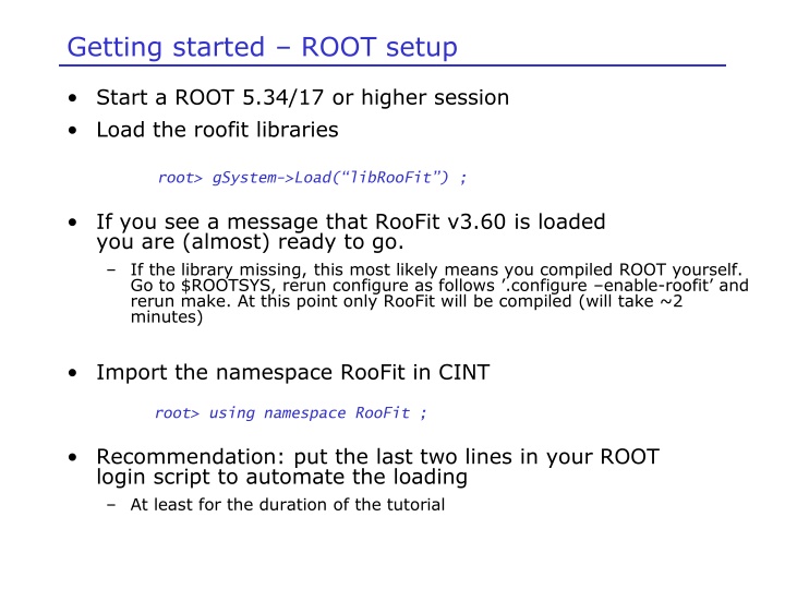
Getting started ROOT setup Start a ROOT 5.34/17 or higher session Load the roofit libraries root> gSystem->Load( libRooFit ) ; If you see a message that RooFit v3.60 is loaded you are (almost) ready to go. If the library missing, this most likely means you compiled ROOT yourself. Go to $ROOTSYS, rerun configure as follows .configure enable-roofit and rerun make. At this point only RooFit will be compiled (will take ~2 minutes) Import the namespace RooFit in CINT root> using namespace RooFit ; Recommendation: put the last two lines in your ROOT login script to automate the loading At least for the duration of the tutorial
Exercise 1 A Poisson counting experiment Untar the file with the exercises, go to the subdirectory set1, and run macro ex1.C. This macro does the following for you: It creates an empty RooFit workspace Fills the workspace a Poisson probability model Poisson(N,S+B) with B fixed to 2, and signal floating (but chosen at 0) It prints the contents workspace: it will show 3 variables (B,N,S) one function object Nexp(B,S) and one probability model model(N,Nexp) . Look at the macro and understand how the variables and function objects are created Plotting the probability model Comment the return statement at the STEP1 comment, and run again. The macro will proceed to make a plot of the probability model for the observable N, for the parameter configuration B=5,S=0 Uncomment the return statement at the STEP2 comment, and run again. The macro will change the value of S from 0 to 2, and plot the distribution of N on the same plot frame
Exercise 2 Maximum Likelihood estimation Say in directory set1/ and run macro ex2.C This macro does the following for you: It recreates the model of ex1 for you (but with less comments) It creates a dataset that contains a (ficticious) measurement of N=7 It creates the log(Likelihood) function for Poisson(N=7|S+B) It plots logL vs the parameter S Q: Does the minimum of log(L) vs S correspond to the estimate of S you expect for N=7? You can zoom in to the minimum by selecting a range in either X-axis or Y- axis on the canvas Performing a maximum likelihood fit Comment the step-1 return statement and let MINUIT minimize the likelihood. Does the minimum correspond to your answer above? MINUIT will also calculate a variance-based uncertainty (HESSE) and a likelihood-ratio interval based uncertainty (MINOS) Measure by eye from your logL-vs-S plot the interval in S around the minimum that is defined by a rise in log(L) of 0.5 units w.r.t the minimum. Does it correspond to the HESSE or MINOS error? Comment the step-2 return statement, and let MINUIT minimize the likelihood for a 2nd observation corresponding to N=10 Optional extra: plot the likelihood for N=10 on top of the existing likelihood curve for N=7
Exercise 3 Compact model expression This is a short technical exercise to learn how to write models more efficiently. Stay in directory set1 and run ex3.C. This macro does the following for you: It recreates the model of ex1 for you (but with less comments) Observing the compact syntax Comment the return statement at step-1 AND comment out the factory expression before return statements (to avoid constructing the same model twice). Observe that the same model is built with compact expression syntax Writing the compact syntax Compactify the model construction to a single line of code by constructing the Nexp function object inline in the factory call that constructs the Poisson model
Exercise 4 Adding a nuisance parameter We will now move to the core topic of this lecture: introducing a systematic uncertainty the model of ex 1 by introducing a subsidiary measurement and a nuisance parameters Stay in directory set1/ and run macro ex4.C This macro does the following for you It makes a slight variation of the model of Ex1, but expresses the signal strength as the product S*mu of the (fixed) nominal signal strength S and a floating signal strength modifier mu (the modifier is then independent of the absolute yield, mu=0 no signal, mu=1 expected signal, mu=2 twice expected signal) Now we introduce a nuisance parameter Make a fit (either using RooMinimizer or using fitTo) that measures the uncertainty on mu, using both HESSE and MINOS. [ Insert code before the Step1 return ] OPTIONAL: Make a plot of logL versus mu in the range [0,2] using your experience of Ex 2.
Exercise 4 continued Now we introduce a nuisance parameter (continued) Now comment the step-1 return statement. Now make a fit of model2 similar to the fit of model before Compare what parameters are fitted, what the fitted values are, and how the uncertainties on the fitted parameters compare What happens to the uncertainty on mu between the 1st and 2nd fit? Congratulations you have just performed your first profile likelihood fit that includes a systematic uncertainty (on the background estimate) in your fitted estimate of mu!
Exercise 5 A sideband measurement We will now explore the similarity between subsidiary measurements and sideband measurements In the model of Ex4 the background rate was constrained by a Gaussian subsidiary measurement that measurement B=20 with an uncertainty of 5 Stay in directory set1/ and run macro ex5.C This macro does the following for you It rebuild the model of Ex 4 in a compact syntax, and fits it to the data Now we rebuild the model assuming that B is measurement in a control region, rather than describing an abstract Gaussian uncertainty Construct a Poisson model for a fictitious control region that measures the model parameter B from an observed number of event NCTL=20 in the control region (Hint: name this model control_model , and name the observable for this control region Nctl and set it to a constant value of 20 Once the control measurement is made, construct a new product (name it model3 of the original measurement model and control_model ) Fit model3 to the data, compared the results
Exercise 5 continued Comparing the results You will find that the uncertainty on mu between the fit to model2 and model3 is somewhat different. This is driven by the fact that the uncertainty on B in both models is also somewhat different: model2 implements a Gaussian uncertainty of width 5, whereas the sideband measurement with Nctl measures and uncertainty of sqrt(20). We have so far assumed that the control region measures the same B as model , but it could very well be that the control region is larger, and would effectively measure twice the rate (i.e. if Nctl =40 then B=20). To introduce this effect of the size of the control region, we introduce an extra (constant) parameter in the model that expresses this rescaling: Construct a new sideband model (name it model_control2) that implements Poisson(Nctl|tau*B) where tau is a constant parameter with value 2. Hint: use an expr::something() function expression to construct an object that represents tau*b . Once this is done, construct a new full model (named model4) that is the product of model and model_control2 and fit this again to the data. What happens to the uncertainty on B and mu? What value of tau should you use to obtain uncertainties on B and tau that are identical to those of model2?
Exercise 6 Multiple nuisance parameters Introducing additional nuisance parameters Stay in directory set1/ and run macro ex6.C This macro does the following for you It rebuild the initial model of Ex 5and fits it to the data Extending the model Currently the main measurement interprets the event rate as Nexp=mu*S+B Modify the model (to your own insight) to describe Nexp=mu*S+B1+B2 where B1 and B2 are two separate (fictitious) source of background. Introduce a Gaussian subsidiary measurement for B1, and a Poisson subsidiary measurement for B2. Explore various values of S and nominal values of B1,B2 and see how this affects the fit (uncertainties, correlations between the fitted parameters) Finally, modify the model to make also S a floating parameter, and add a 3d subsidiary measurement that constrains the (now floating) parameter S to its nominal value Fit again this model and look if you understand the fitted values, uncertainties and correlations between model parameters (also compared to the previous fit)
Exercise 7 Beyond counting experiments The concept of introducing systematic uncertainties extends equivalently to fits to distributions of data (instead of event counts explored so far) Stay in directory set1/ and run macro ex7.C This macro does the following for you: It builds an extended unbinned likelihood fit that describes the shape of a distribution. It has a similar structure to previous excercises (a signal component with expected yield S and a background component with yield B) It plots the distribution of the observed data in observable x, along with the model prediction for this observable Introducing nuisance parameters in a shape fit Make the (now-fixed) B parameter a floating parameter and fit again. You will observe that since this is a shape fit B can be constrained from the measurement, and a subsidiary measurement is not needed (like it was for the counting measurement)
Exercise 7 Beyond counting experiments Introducing nuisance parameters in a shape fit Nevertheless, it is possible that B could measurement by a subsidiary measurement with a higher precision that the main measurement: Introduce a high-precision Gaussian subsidiary measurement for B with a value that is consistent with the best-fit value so far, and an uncertainty that is 3x smaller than the best- fit value. How does this affect the measurement value and uncertainty of mu? What happens if you increase the background by a factory 10? Next, also make the width of the Gaussian signal a nuisance parameter, similar to B: first make width a floating parameter, then add a subsidiary measurement that constrains the width to one-tenth of the precision of the main measurement. Finally, observe what happens if the subsidiary measurement of width constrains the parameter width with high precision to a value that is inconsistent with the main measurement (e.g. introduce a subsidiary measurement that measures width = 3 +/- 0.1)
5 A very short course on practical course RooFit Mathematical objects are represented as C++ objects Mathematical concept RooFit class x (x variable RooRealVar ) f function RooAbsReal (x x ) f PDF RooAbsPdf space point RooArgSet x x min max ( dx ) f x integral RooRealIntegral list of space points RooAbsData
6 Every function, variable etc is a separate C++ object Example: all components needed to form a Gaussian probability model Gauss(x, , ) Math RooGaussian g RooFit diagram RooRealVar x RooRealVar y RooRealVar z RooFit code RooRealVar x( x , x ,-10,10) ; RooRealVar m( m , y ,0,-10,10) ; RooRealVar s( s , z ,3,0.1,10) ; RooGaussian g( g , g ,x,m,s) ;
8 Factory and Workspace One C++ object per math symbol provides ultimate level of control over each objects functionality, but results in lengthy user code for even simple macros Solution: add factory that auto-generates objects from a math-like language Gaussian::f(x[-10,10],mean[5],sigma[3]) RooRealVar x( x , x ,-10,10) ; RooRealVar mean( mean , mean ,5) ; RooRealVar sigma( sigma , sigma ,3) ; RooGaussian f( f , f ,x,mean,sigma) ;
Populating a workspace the easy way the factory Creating many objects can be tedious: The workspace factory allows to fill a workspace with pdfs and variables using a simplified scripting language Gauss(x, , ) Math RooWorkspace RooWorkspace RooAbsReal f RooFit diagram RooRealVar x RooRealVar y RooRealVar z RooFit code RooWorkspace w( w ) ; w.factory( RooGaussian::g(x[-10,10],m[-10,10],z[3,0.1,10]) );
9 Factory and Workspace This is not the same as reinventing Mathematica! String constructs an expression in terms of C++ objects, rather than being the expression Objects can be tailored after construction through object pointers For example: tune parameters and algorithms of numeric integration to be used with a given object Implementation in RooFit: Factory makes objects, Workspace owns them RooWorkspace w( w ,kTRUE) ; w.factory( Gaussian::f(x[-10,10],mean[5],sigma[3]) ) ; w.Print( t ) ; variables --------- (mean,sigma,x) p.d.f.s ------- RooGaussian::f[ x=x mean=mean sigma=sigma ] = 0.249352
10 Accessing the workspace contents Contents can be accessing in two ways Through C++ namespace corresponding through w space Super easy (NB: does not always work on MS Windows) But works in ROOT interpreted macros only RooWorkspace w( w ,kTRUE) ; w.factory( Gaussian::g(x[-10,10],0,3) ) ; w::g.Print() ; Through accessor methods A bit more clutter, but 100% ISO compliant C++ (and compilable) RooAbsPdf* g = w.pdf( g ) ; RooRealVar* x = w.var( x ) ;
11 Factory language The factory language has a 1-to-1 mapping to the constructor syntax of RooFit classes With a few handy shortcuts for variables Creating variables x[-10,10] // Create variable with given range, init val is midpoint x[5,-10,10] // Create variable with initial value and range x[5] // Create initially constant variable Creating pdfs (and functions) Gaussian::g(x,mean,sigma) Polynomial::p(x,{a0,a1}) RooGaussian( g , g ,x,mean,sigma) RooPolynomial( p , p ,x ,RooArgList(a0,a1)); Can always omit leading Roo Curly brackets translate to set or list argument (depending on context)
12 Factory language Composite expression are created by nesting statements No limit to recursive nesting Gaussian::g(x[-10,10],mean[-10,10],sigma[3]) x[-10,10] mean[-10,10] sigma[3] Gaussian::g(x,mean,sigma) You can also use numeric constants whenever an unnamed constant is needed Gaussian::g(x[-10,10],0,3) Names of nested function objects are optional SUM syntax explained later SUM::model(0.5*Gaussian(x[-10,10],0,3),Uniform(x)) ;
12 Factory language Interpreted function expressions allow to customize existing probability density functions // construct Nexp=mu*S+B (a function) expr::Nexp( mu*S+B ,mu[0,5],S[50],B[50]) // construct a Poisson probability model describing // the distribution of Nobs given Nexp Poisson::p(Nobs[0,1000],Nexp) ; Generally: types starting with upper-case are Probability Density Functions, types starting with lower-case are simple functions expr is a special function type that implements an interpreted C++ function
21 Model building (Re)using standard components List of most frequently used pdfs and their factory spec Gaussian Gaussian::g(x,mean,sigma) Breit-Wigner BreitWigner::bw(x,mean,gamma) Landau::l(x,mean,sigma) Exponental::e(x,alpha) Polynomial::p(x,{a0,a1,a2}) Chebychev::p(x,{a0,a1,a2}) Landau Exponential Polynomial Chebychev Kernel Estimation KeysPdf::k(x,dataSet) Poisson Poisson::p(x,mu) Voigtian Voigtian::v(x,mean,gamma,sigma) (=BW G)
13 Basics Creating and plotting a Gaussian p.d.f Setup gaussian PDF and plot // Build Gaussian PDF w.factory( Gaussian::gauss(x[-10,10],mean[-10,10],sigma[3,1,10] ) // Plot PDF RooPlot* xframe = w.var( x )->frame() ; w.pdf( gauss )->plotOn(xframe) ; xframe->Draw() ; Axis label from gauss title Unit A RooPlot is an empty frame capable of holding anything plotted versus it variable normalization Plot range taken from limits of x
14 Basics Generating toy MC events Generate 10000 events from Gaussian p.d.f and show distribution // Generate an unbinned toy MC set RooDataSet* data = w.pdf( gauss )->generate(w::x,10000) ; // Generate an binned toy MC set RooDataHist* data = w.pdf( gauss )->generateBinned(w::x,10000) ; // Plot PDF RooPlot* xframe = w.var( x )->frame() ; data->plotOn(xframe) ; xframe->Draw() ; Can generate both binned and unbinned datasets
16 Basics ML fit of p.d.f to unbinned data // ML fit of gauss to data w.pdf( gauss )->fitTo(*data) ; (MINUIT printout omitted) PDF automatically normalized to dataset // Parameters if gauss now // reflect fitted values w.var( mean )->Print() RooRealVar::mean = 0.0172335 +/- 0.0299542 w.var( sigma )->Print() RooRealVar::sigma = 2.98094 +/- 0.0217306 // Plot fitted PDF and toy data overlaid RooPlot* xframe = w.var( x )->frame() ; data->plotOn(xframe) ; w.pdf( gauss )->plotOn(xframe) ;
17 Basics ML fit of p.d.f to unbinned data Can also choose to save full detail of fit RooFitResult* r = w::gauss.fitTo(*data,Save()) ; r->Print() ; RooFitResult: minimized FCN value: 25055.6, estimated distance to minimum: 7.27598e-08 coviarance matrix quality: Full, accurate covariance matrix Floating Parameter FinalValue +/- Error -------------------- -------------------------- mean 1.7233e-02 +/- 3.00e-02 sigma 2.9809e+00 +/- 2.17e-02 r->correlationMatrix().Print() ; 2x2 matrix is as follows | 0 | 1 | ------------------------------- 0 | 1 0.0005869 1 | 0.0005869 1
Exercise 10 Template fits We will now construct a first template fit, where a signal and a background model are described by a histogram obtained from MC simulation Change to directory set2/ and run ex10.C Note that this macro uses input file ex10.root This macro does the following for you It opens ex10.root and uses the a template histogram in ex10.root to construct a probability model for signal in an observable x Performing a simple template fit Open first ex10.root and look at the TH1 histograms stored in here: there is a signal template, a background template and a data histogram In a new root session, run macro ex10.C. You now see the signal histogram used to construct a yield function (a RooHistFunc) in. Add code to also do this for the background template (the TH1 is called h_bkg, name the corresponding RooDataHist and RooHistFunc dh_bkg and fh_bkg respectively)
Exercise 10 Performing a simple template fit Now construct from the sum of two yield functions a probability model as follows (in the workspace factory) ASUM::model(mu[1,0,5]*hf_sig,nu[1]*hf_bkg) This class takes two yield histograms and turns the weighted sum of these in a probability model that can fitted. Fit the model to the data, make a plot of the data overlaid with the fitted model (hint: first call data.plotOn(frame) and then model.plotOn(frame). You can also overlay the background component of the model as shown in set1/ex7.C) OPTIONAL: repeat this exercise with different templates and datasets to observe how signal/background shape and yields affect the fitted signal rate mu. To make these modified inputs, copy file set2/makeinput/makeinput_ex10.C, adjust the parameters inside it, and run it to regenerate ex10.root
Exercise 11 (Optional, skip if you are short on time!) Performing a template fit accounting for MC statistical uncertainties Beeston-Barlow-style Stay in directory set2/ and run file ex11.C Note that this macro uses input file ex11.root Note that this macro also compiles two custom classes that are located in the directory set2/code. If your ROOT setup does not allow on-the-fly compilation of code ( .L myclass.cxx+ ) you should skip this exercise This macro does the following for you When you run the macro for the first time (only) it will compile classes RooParamHistFunc2 and RooHistConstraint2 for you These classes fix a small bug in the corresponding classes in the distribution that would otherwise affect this tutorial. It opens ex11.root and uses the template histograms in ex11.root to construct a probability model for signal plus background in an observable x Note that the number of bins has changed from 100 to 20 A template fit accounting for statistical uncertainties Perform a fit of the model to the data dataset and plot the dataset and model overlaid, following the example of ex10. Now change the rigid template for signal and background in a flexible template for signal and background as follows:: change class HistFunc in class ParamHistFunc2 (don t forget the trailing 2 in the class name!) When you fit again you will that result is (still) the same, as parameters that can change each bin the templates are initially constant.
Exercise 11 (Optional, skip if you are short on time!) A template fit accounting for statistical uncertainties Now we need to construct the classes that introduces the subsidiary Poisson measurements that constrain the parameters of the flexible template parameters to the measured MC event counts: HistConstraint2::hc_sig(hf_sig) The only constructor argument is the template function (RooParamHistFunc, named hf_sig in the code example above) for which it makes subsidiary measurement. (The construction of this subsidiary measurement will automagically make all parameters of the RooHistFunc2 floating ) Construct objects of type HistConstraint2 for both the signal and background template (name them hc_sig and hc_bkg) Finally, construct the full model multiplying the template model and the two HistConstraint2 objects (use PROD::model2( .) to construct the product, similar to Ex4. Note that you can use one PROD() object to multiply any number of models Fit the template model2 that now includes Beeston-Barlow MC statistical uncertainty treatment. Look at the values of all fit parameters and in particular compare the uncertainty on mu of this fit w.r.t. the earlier fit to the rigid template model. Is the difference between mu uncertainties consistent with your expectation?
Exercise 11 A template fit accounting for statistical uncertainties We can now vary the number of observed events in the fit to judge the relative importance of treating MC statistical uncertainties To do that we must first modify the model to account for the fact that the number of data events is different from the sum of the number of template events: extend the ksig/kbkg scale factor functions to include a third term SF[1] to introduce an additional constant scale factor that is (for now) 1. Fit again to confirm that the modified model including the (now-unit) scale factor gives the same answer. Now set the scale factor SF to 0.1 and fit data_small instead of data . The uncertainty on mu will increase as the data sample is small Now set the scale factor SF to 10 and fit the data_large sample. The uncertainty on my will decrease as the sample is large. Finally, comment out the lines of code that construct the RooHistConstraint objects and the line that constructs model2 (using PROD). This will revert model to the rigid template mode . Now fit model (instead of model2) and observe the uncertainty when MC statistical uncertainties are not taken into account. How big is the uncertainty on mu due to MC template uncertainties?
Exercise 12 Constructing a template morphing model that accounts for a jet energy scale (JES) uncertainty in the signal template Stay in directory set2/ and run macro ex12.C What does this macro do for you? It opens ex12.root and uses the a template histogram in ex12.root to construct a probability model for signal plus background in an observable x Note that we switched back to 100 bins for a more dramatic visualization Constructing a template morphing model Run the macro as provided and observe the fit result and plotted result. The first step towards setting up a template morphing model is constructing HistFunc objects for the JES-up and JES-down variation templates (the datasets are already imported by the macro) The next step is to make a template morphing signal model. The magic class to do this is called PiecewiseInterpolation PiecewiseInterpolation:pi_sig(Fnom,Flo,Fhi,NP) where Fnom/lo/hi are the RooHistFuncs representing the nominal, down and up templates and NP is the nuisance parameter associated with the systematic uncertainty. Construct the PiecewiseInterpolation function, and the nuisance parameter (call that one alpha with a range [-5,5]).
Exercise 12 Constructing a template morphing model Make a 2D plot of the template morphing signal model in the observable x and the nuisance parameter alpha w::pi_sig.createHistogram( x,alpha )->Draw( SURF ) You will clearly see that in the default configuration the signal model is allowed to extrapolate to negative signal yields. Disable this feature (w::pi_sig.setPositiveDefinite(kTRUE)) and remake the above plot You also clearly see the kinks in the predictions at alpha=0, as the model by default implements a piece-wise linear model. Switch this to polynomial interpolation model (w::pi_sig.setAllInterpCodes(4)) and remake the above plot. Finally construct the full template morphing model by 1) replacing in the model , the simple signal model hf_sig with the morphing model pi_sig 2) constructing the full likelihood model2 as the product of model and Gaussian subsidiary measurement on alpha (with observed value 0 and width 1) Fit the template morphing model to the data and observe the effect of the introduction of the JES uncertainty on mu. Also look at the fitted value of alpha and its uncertainty. Is the physics measurement able to constrain the JES uncertainty beyond the input of the subsidiary measurement?
Exercise 13 Extend the template morphing model to two uncertainties: Copy set2/makeinput/makeinput_ex13.C to set2/, which make two additional templates corresponding to a signal width variation Copy your solution to ex12.C to ex13.C. Import the width variation templates (corresponding to a Jet Energy Resolution systematic uncertainty) in ex13.C Modify the PiecewiseInterpolation::pi_sig to morph in two dimensions. The constructor syntax for 2 (or more) dimensions is PiecewiseInterpolation::pi_sig(nom,{down_a,down_b},{up_a,up_b}, {np_a,np_b}) ; where down_(a,b) and up_(a,b) are RooHistFuncs, and np_(a,b) are the corresponding Nuisance Parameters. Call the nuisance parameter for resolution morphing beta. Extend model2 to include a Gaussian subsidiary measurement for beta, and rerun the fit.
Exercise 14 - Optional Having an easy time so far? Include the effect MC statistical uncertainties in the template morphing model of ex12 First change the number of bins to 20, to reduce number of parameters. In set2/makeinput/makeinput_ex12.C introduce a call to w::x.setBins(20) just after the workspace is filled. Then in ex12.C, make the same modification, andmodify the binw[1] to binw[0.2] . Rerun to confirm that everything still works OK Include the two gROOT->ProcessLine() statements from ex11.C to load the required classes for Beeston-Barlow modelling Now introduce the effect of MC statistical uncertainties on the background model. This one is the easiest, since it is not modified w.r.t ex10. You change the HistFunc in a ParamHistFunc2 and you include the corresponding HistConstraint2 object in the list of subsidiary measurements. Run the fit Next you introduce the effect of MC statistical uncertainties on the central template of the signal model. This is only marginally more complicated: you simply replace the central template that goes into the PiecewiseInterpolation model with a ParamHistFunc2 version. Then, just like above, you add the corresponding HistConstraint2 object to the list of subsidiary measurements. Run the fit


")
")