Goodness of Fit and Contingency Tables in Statistics
This content discusses the importance of testing a model's fit with observed data, using expected vs. observed frequencies to determine goodness of fit, and the concept of the chi-squared distribution in statistical analysis. It highlights the process of assessing whether assumptions made in modeling are supported by the data, offering insights into hypothesis testing and model evaluation in statistics.
Download Presentation

Please find below an Image/Link to download the presentation.
The content on the website is provided AS IS for your information and personal use only. It may not be sold, licensed, or shared on other websites without obtaining consent from the author.If you encounter any issues during the download, it is possible that the publisher has removed the file from their server.
You are allowed to download the files provided on this website for personal or commercial use, subject to the condition that they are used lawfully. All files are the property of their respective owners.
The content on the website is provided AS IS for your information and personal use only. It may not be sold, licensed, or shared on other websites without obtaining consent from the author.
E N D
Presentation Transcript
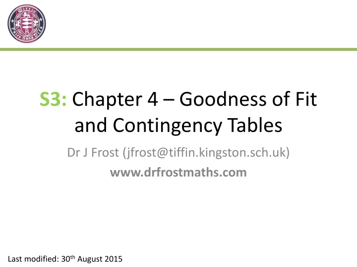
S3: Chapter 4 Goodness of Fit and Contingency Tables Dr J Frost (jfrost@tiffin.kingston.sch.uk) www.drfrostmaths.com Last modified: 30th August 2015
Testing a Model Going back to Chapter 1 of S1 (that chapter that every teacher skips), we had the idea of modelling: Simplifying assumptions Data Model e.g. Collected heights of people in the population e.g. Normal distribution using ? and ?2 from data. Why might we want to use a model for a data? It often makes calculations from the data easier, e.g. for heights in the population, if we assume a Normal Distribution, we could then calculate probabilities of someone having a given height range. This might be difficult if we used the raw data. ? This chapter mostly concerns how well a chosen model fits the observed data. If our simplifying assumptions were justified, we should find the model is a good fit.
Expected Frequency vs Observed Frequencies I throw a die (which may be fair) 120 times and observe the counts of each possible number. Number 1 2 3 4 5 6 Observed Freq, ?? Expected Freq if fair die, ?? 23 15 25 18 21 18 20 20 20 20 20 20 ? An obvious thing we might want to do is hypothesise whether or not the die is fair based on the counts seen. We need some sensible way to measure the difference between the observed and expected frequencies. Bronotation note: ?2 is a standalone symbol rather than something squared. ? would never be used on its own. It just gives an indication the differences between the counts is squared. Measure of goodness of fit: ? ?? ?? 2 2 = ?? ?2= ? ? ? ?? ?? ?=1 Why the ??? It has a normalising effect, so that the (squared) difference is given as a proportion of the expected frequency. ? Why the squared? It ensures difference is positive. ?
?2(Kye squared) distribution Number 1 2 3 4 5 6 Observed Freq, ?? Expected Freq if fair die, ?? 23 15 25 18 21 18 20 20 20 20 20 20 Suppose we standardised this normal distribution (representing the possible observed frequencies for one particular outcome), so that 0 means the observed frequency is equal to the expected frequency, and that we square this random variable to ensure the difference is positive. Suppose that the die was indeed fair. If we threw another 120 times, collected counts, and repeated again and again, then for say the outcome of 1, we d expect a distribution of possible counts centred around 20; indeed if ?? is large then by the CLT these possible observed frequencies is approximately normally distributed. Possible observed counts (now standardised and squared) i.e. possible deviation of the observed frequency from the expected frequency Then if we summed these normal distributions for each outcome, we d obtain a new distribution representing the total possible (standardised) deviations of the observed frequencies from expected frequencies. This is known as the ?? distribution. Rather handily ?? (our goodness of fit measure) is approximately distributed as ??provided the expected frequencies are large (rule of thumb: 5) 20 Possible observed counts given that expected count is 20.
Degrees of Freedom The ?2 distribution has one parameter: degrees of freedom (? Greek Letter nu ), which is how many values we have that can vary. Number 1 2 3 4 5 6 Observed Freq, ?? 23 15 25 18 21 18 Degrees of freedom in this example = 5 (given that ? is fixed) ? The counts for 1 through to 5 can vary, however, the count for the remaining outcome 6 is determined by the other counts (i.e. ? minus the other counts). The constraint that the outcomes add up to ? removes a degree of freedom. The number of degrees of freedom ? = number of cells number of constraints So when in combining the normal distributions for each outcome to give some kind of total measure of possible deviation of observed frequencies from expected frequencies, it doesn t make sense to add another normal distribution for the last outcome, because the observed frequency can t actually vary! (which goes against the notion of a random variable )
Example: Hypothesis Testing Number 1 2 3 4 5 6 Observed Freq, ?? Expected Freq, ?? 23 15 25 18 21 18 20 20 20 20 20 20 Test, at the 5% significance level, whether or not the observed frequencies could be modelled by a discrete uniform distribution. ? ?0: The observed distribution can be modelled by a discrete uniform distribution (i.e. die is not biased) ?1:The observed distribution cannot be modelled by a discrete uniform distribution (i.e. die is biased) ? = ? Critical value of ?2 at 5% level: ??.??? ? ? Look up in ?? table. If our goodness of fit measure is this value or worse (i.e. observed frequencies deviate too much from expected frequencies) then we ll be able to conclude that die was biased. Number 1 2 3 4 5 6 Total ?? 23 15 25 18 21 18 120 ?? 20 20 20 20 20 20 120 ? 0.45 1.25 1.25 0.2 ? 0.05 0.2 3.4 ?? ?? ?? ? ? Critical region Since 3.4 < 11.070 we do not reject ?0. There is no evidence that the die is biased. 5% ?25 3.4 11.070
Test Your Understanding A 3-sided spinner is spun 150 times, and counts of the three outcomes are shown. Test, at the 1% significance level, whether or not spinner is fair. Number 1 2 3 Total Observed 35 60 55 150 ?0: The observed distribution can be modelled by a discrete uniform distribution (i.e. die is not biased) ?1: The observed distribution cannot be modelled by a discrete uniform distribution (i.e. die is biased) ? = 2 Critical value of ?2 at 1% level: 9.210 ? Number 1 2 3 Total ?? 35 60 55 150 ?? 50 50 50 150 ? 4.5 2 0.5 7 ?? ?? ?? 7 < 9.210 so we do not reject ?0. Cannot conclude that the spinner is biased.
General Method for Goodness of Fit We have so far tested against a discrete uniform distribution, but we can obviously test against any other distribution in exactly the same way. Testing for goodness of fit: 1. Determine which distribution would conceptually be most appropriate (e.g. Binomial, Poisson). 2. Set significance level. 3. Estimate parameters (if necessary) from observed data. 4. Form hypotheses ?0 and ?1 5. Calculate expected frequencies. 6. Combine any expected frequencies so that none are < 5 7. Find degrees of freedom. 8. Find critical value of ?2 from table. ?? ?? ?? 10. See if value is significance and draw conclusion. 2 2 or ?? 9. Calculate ?? ?
Testing a Binomial Distribution as Model The data in the table is thought to be modelled by a binomial ?(10,0.2). Use the table for the binomial cumulative distribution function to find expected values, and conduct a test to see if this is a good model. Use a 5% significance level. ? 0 1 2 3 4 5 6 7 8 Freq of ? 12 28 28 17 7 4 2 2 0 ?0: A ?(10,0.02) distribution is a suitable model for results. ?1: Distribution is not suitable. ? = 100 ? Bro Tip: You can use tables and find differences to retrieve probabilities. ? ? 0 ? ? 1 2 3 4 5 6 ? ? 7 8 ? ? 0.2684 ? ? 0.3020 ? ? 0.2013 ? ? 0.0881 ? ? 0.0264 ? ? 0.0008 ? ? ? ? 0.1074 0.0055 0.0001 Expected freq 10.75 26.84 30.20 20.13 8.81 2.64 0.55 0.08 0.01 Recall that our expected frequencies need to be 5. So combine by adding. ?? 12 28 28 17 15 ? ? ? = 4(?was not estimated by calculation so it s just 5-1) ?2= 1.5453 1.5453 < 9.488 so do not reject ?0. ? 10,0.02 is a possible model for the data. ? ? ?? 10.74 26.84 30.20 20.13 12.09 ? ? 0.1478 0.0501 0.1603 ? 0.4867 0.7004 ?? ?? ??
When ? is not given A study of the number of girls in families with five children was done on 100 such families. The results are summarised in the following table. Num girls ? 0 1 2 3 4 5 Freq (?) 13 18 38 20 10 1 Test, at the 5% significance level, whether or not a binomial distribution is a good model. ?0: A binomial distribution is a suitable model. ?1: It is not a suitable model. Number of observations ? = 100 ? ? = 5 ? ? =? ? ? 199 = 100 5= ?.??? ?? Because we estimated ?, there are TWO constraints. ? ? 0 1 2 3 4 5 0 1 2 3 >3 Total 0.2285 ? ?(?) ?? 0.0791 0.2614 0.3456 0.0755 0.0099 13 18 38 20 11 ? ?? ?? 7.91 26.14 34.56 22.85 ? 8.54 7.91 26.14 34.56 ? 22.85 7.55 0.99 2 21.37 12.39 41.78 17.51 14.17 107.22 ?? ?? ? = 5 2 = 3 Critical value is ?3 ? 2= 7.815 2 ?? ?? ? ? = ? 7.22 < 7.815 You do not reject ?0. Binomial is a suitable model. ? ? = 107.22 100 = 7.22
Quickfire ? and ? The easiest way to remember how to calculate ? is to find the mean of the table and then divide by the ? of the Binomial. Num squirrels ? 0 1 2 ? =?.? = ?.? ? ? ? = ? ? = ? ? Freq (?) 3 2 5 Dice outcome (?) 0 1 2 3 ? =?.?? ? = ?.??? ? ? = ? ? = ? ? Freq (?) 4 1 5 10
Test Ye Understanding S3 May 2012 Q6 ? ?
Testing a Poisson Distribution as Model The numbers of telephone calls arriving at an exchange in six-minute periods were recorded over a period of 8 hours, with the following results. Num calls ? 0 1 2 3 4 5 6 7 8 Freq (?) 8 19 26 13 7 5 1 1 0 Can these results be modelled by a Poisson distribution? Test at the 5% significance level. ?0: A Poisson distribution is a suitable model for number of calls. ?1: It is not a suitable model. Number of observations ? =? ?? ? = ?? ? An estimate for ? is simply the mean number of calls! (by definition of ?) ? ? =??? ??= ?.? ? ?(?) ? Expected freq of ? ? ? ? 2 ? ?? ?? ?? ?? ?? ? = ? ? = ? ?4 0.1108 80 = 8.864 0 0.1108 ? 25% = ?.??? 1 0.2438 19.504 8.864 0 8 0.0842 2 0.2681 21.448 1 19 19.504 0.0130 ? 2.1016 > 9.488 So you have no evidence to reject ?0 Calls may be modelled by ??(2.2) distribution. ? 3 0.1966 15.728 ? 2 26 21.448 0.9661 4 0.1082 8.656 3 13 15.728 0.4732 5 0.0476 3.808 4 7 8.656 0.3168 6 0.0174 ? 1.392 ? 5 7 3.808 0.2483 7 0.0075 0.6 Just 1- the rest.
Goodness of Fit Tests for Continuous Distributions We might want to test how our data fits a normal distribution. Clues that data is normally distributed: Data centred about mean. Approximately 68% of data fall within one standard deviation of the mean (remember the 68-95-99.7 rule?). ? Parameters that may be given or may need to be estimated: ?,? ? How does this affect ?? We have to deduct one degree of freedom for each parameter estimated. ?
Example During observations on the height of 200 male students the following data were observed: Height (cm) 150-154 155-159 160-164 165-169 170-174 175-179 180-184 185-189 190-194 Freq 4 6 12 30 64 52 18 10 4 a. Test at the 0.05 level to see if the height of male students could be modelled by a normal distribution with mean 172 and standard deviation 6. b. Describe how you would modify this test if the mean and variance were unknown. How do you think we would find the probability of the 155-159cm range? Just find ? ???.? < ? < ???.? How about the 150-154 range? ?(? < ???.?), as if we didn t include below 149.5, our probabilities wouldn t sum to 1. ? ? ? ? ? ? ? ? Classes (? ?) ?? ? ? ? ? ? ? ? ? ? ? ? ? < ? = ? ? 0.38 ? ? ? < 154.5 2.92 0.0019 0.0000 = 0.0019 Notice that by calculating the z- probability for the upper bound each time, we can reuse it as the lower bound in the next range. 154.5 159.5 2.08 0.0188 0.0019 = 0.0169 3.38 159.5 164.5 1.25 0.1056 0.0188 = 0.0868 17.36 ? 0.38 ? 1.0000 0.9981 = 0.0019 ? > 189.5
Example During observations on the height of 200 male students the following data were observed: Height (cm) 150-154 155-159 160-164 165-169 170-174 175-179 180-184 185-189 190-194 Freq 4 6 12 30 64 52 18 10 4 a. Test at the 0.05 level to see if the height of male students could be modelled by a normal distribution with mean 172 and standard deviation 6. b. Describe how you would modify this test if the mean and variance were unknown. Estimate parameters: ? = ???? ?? ????? ?2= ?????? ???????? ? = 5 3 = 2 ? We have three constraints! ? is fixed, ? is fixed, ? is fixed.
Test Your Understanding June 2013 Q4 (Note that this table does NOT have gaps) a ? b ? c ?
Continuous Uniform Distribution Recap: If we have a continuous uniform distribution in the range ?,? , i.e. ?~? ?,? , then what is ? ? < ? < ? ? ? ? ? ? ? ? < ? < ? =? ? ? ? ?
Example Question In a study on the habits of a flock of starlings, the direction in which they headed when they left their roost in the mornings was recorded over 240 days. The direction was found by recording if they headed between certain features of the landscape. The compass bearings of these features were than measured. The results are given below. Suggest a suitable distribution, and test to see if the data supports this model. 0 ? < 58 100 ? < 127 127 ? < 190 58 ? < 100 190 ? < 256 256 ? < 296 296 ? < 360 Direction (degrees) 31 40 47 40 32 30 20 Frequency 58 360= 0.1611 ? ? ? ? < ? < ? 0.1167 ? ? 0.075 0.0175 0.1833 ? ? 0.1111 0.1778 ? 38.67 28 18 42 44 26.66 42.67 Continuous uniform distribution suitable as frequencies are symmetrical about mean and we d expect frequencies to be roughly the same where class widths are the same. Why possibly suitable ? ?0: Continuous uniform distribution suitable model ?1: Not a suitable model ? = 7 1 = 6 (not parameters were estimated) ?2= 69.2171 69.2171 > 12.592 therefore reject ?0. Birds do not feed in all directions they have preferred feeding areas. ? ? ? ?
Test Your Understanding June 2010 Q6 ?
Contingency Tables Grade ? ? ? Totals ? School 18 12 20 50 ? 26 12 32 70 Totals 44 24 52 120 So far, we have repeated a single event to get counts, e.g. throwing a single die multiple times, or in this case sampling grades from a single school and taking counts of each grade. We then determined how well this fit a particular distribution (uniform, binomial, etc.) But we might have multiple sets of results, and want to instead see how independent school and grade are did say pupils in school A receive better teaching, or was the difference just due to chance? (i.e. natural variability) This table is known as a ? ? contingency table (rows first, then columns, just like matrices).
Contingency Tables Determine to the 5% significance level whether school and grade are dependent. Grade ? ? ? Totals ? School 18 12 20 50 ? 26 12 32 70 Totals 44 24 52 120 i.e. there is not any association between the two criterion ?0: School and grade are independent. ?1: School and grade are not independent ? Using the totals, what is the probability that a student is from school ? and has a grade ?? 44 120 50 120 ? ? ? ? = Hence what is the expected number of students from school ? getting grade ?? 44 120 50 120 120 =44 50 ? 120 Expected frequency =??? ????? ?????? ????? ????? ?????
Contingency Tables Grade ? ? ? Totals ? School 18 12 20 50 ? 26 12 32 70 Totals 44 24 52 120 Expected Frequencies Grade ? ? ? Totals 50 44 120 70 44 120 44 50 24 120 70 24 120 24 50 52 120 70 52 120 52 ? School 50 = 18.33 ? ? = 21.67 ? = 10 ? 70 = 25.67 ? ? = 30.33 ? = 14 Totals 120
Contingency Tables Grade ? ? ? Totals ? School 18 12 20 50 ? 26 12 32 70 Totals 44 24 52 120 Degrees of Freedom for ? table? i.e. Given the fixed totals, how many cells could you fill in before all other values could be determined? ? = ( 1)(? 1) ? ? In this example ? = 2 1 3 1 = 2
Contingency Tables ? ?? ?? ?? ?? 18 18.33 17.676 12 10.00 14.4 20 21.67 18.46 26 25.67 26.334 12 14.00 10.286 32 30.33 33.76 ? ? ?2= 120.916 120 = 0.916 ?2 2= 5.991 0.916 < 5.991 so do not reject ?0. Insufficient evidence to suggest an association between school and grade of pass the two are independent. ?
Test Your Understanding June 2010 Q5 ?
Exercise 4D Question 4 onwards.
