Graphical Models in Bayesian Networks: Examples and Concepts

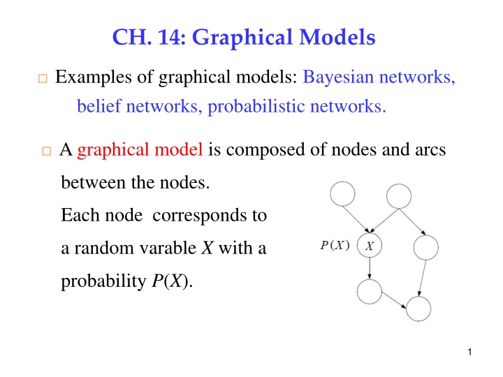
CH. 14: Graphical Models Examples of graphical models: Bayesian networks, belief networks, probabilistic networks. 1 A graphical model is composed of nodes and arcs between the nodes. Each node corresponds to a random varable X with a probability P(X). 1

Adirected arc from nodes X Y (X: parent, Y: child) is specified by the conditional probability P(Y | X). 14.1 Introduction Graphical models help to infer over a large number of variables by decomposing the inference into a set of local calculations each involving a small number of variables 2

Given the graphical model of the random variables their joint probability is calculated by 1, , , X X 3 n n ( ) = , , ( |Parents( )) P X X P X X 1 n i i = 1 i Example 1: ( = ) , , , , P X X X X X 1 2 3 4 5 ( ( ( ) ( | X ) ( P X P X ) | , P X P X X X 1 2 3 1 2 ) ( , X ) | P X X 4 2 5 3 ) | P X X 6 4 5 3

Example 2: Causal and Diagnostic inferences Given: 4 = ( ( ( : : ) 0.6, = P P P R W R W | ) | : 0.1, 0.8 = : ) R ( ) The joint probability: = , ( ) ( P R P W R | ) P R W The marginal (individual) probability: ( ) ( ) = , P W P R W R 4

( ) P W ( ) = = + , ( ) ( P R P W R | ) ( : ) ( R P W | : ) P R W P R R = 0.4 0.9 + 0.6 0.2 = 0.48 Causal inference : explains the cause of W is R ( | ) P W R Diagnostic inference ( | P R W ) From Bayes rule, ) ( ) ) P W 0.9 0.4 0.48 ( | P W R P R ( ) = | P RW ( = = 0.75 5

X and Y are independent if P(X,Y) = P(X)P(Y) From conditional probability ( ( , ) ( | ) ( ). If and are independent, ( , ) ( , ) ( | ) ( ) ( ) ( | ) ( ) P X P X Y P Y = = | ) ( , )/ ( ), P X Y P X Y P Y 6 = P X Y X P X Y P X Y P Y = ( ) ( ). Y P X Y P X P Y = P X P Y = ( ) ( ) P X Y P Y X and Y are conditionally independent given Z if P(X,Y|Z) = P(X|Z)P(Y|Z) or P(X|Y,Z) = P(X|Z) Forming a graphical model by adding nodes (according to random variables) and arcs (according to dependencies of variables). 6

14.2 Three Canonical Cases for Conditional Independence 7 Case 1: Head-to-Tail -- X is the parent of Y and Y is the parent of Z. Joint Probability: P(X,Y,Z) = P(X)P(Y|X)P(Z|Y) ( P X Y ) ( ) , , ) ( | ( P X P Y X ) ( | P X Y Z P X P Y X P Z Y ( ) = = Q | , P Z X Y ( , ) ) ( | = ) ( | ) P Z Y conditional probability joint probability X and Z are conditional independent given Y 7

Example: 8 ( ) P R = = + ( | ) ( ) P R C P C ( | ) ( ) P R C P C ( | P R : ) ( : ) C P C C = 0.8 0.4 0.1 0.6 + = ( ) P W 0.38 = = + ( | ) ( ) ( | ) ( ) ( | : ) ( R P : ) P W R P R P W R P R P W R R = 0.9 0.38 0.2 0.62 + = 0.47 = ( | ) | ) ( | ) P W R P R C ( P W C R P W R P R C = = + = | ) ( | ) 0.9 0.8 0.2 0.2 + ( ( | : ) ( R P : | ) P W R C 0.76 8

( | ) ( ) ( ) P W 0.76 0.4 0.47 P W C P C = = = ( | P C W ) 0.65 9 Case 2: Tail-to-Tail -- X is the parent of two nodes Y and Z. Joint Probability: ( , , P X Y Z ) ( ) = ) ( | ) ( | P X P Y X P Z X Given X, Y and Z become independent. ( , | P Y Z X P X ) ( ) , , ( ) ( | ) ( | ) ) ( | P X Y Z P X P Y X P Z X P X = ( ) = = Q ) ( ( | P Y X P Z X ) conditional probability joint probability 9

Example: ( | ) ( ) ( ) P R P R C P C ( ) = | P C R 10 ( | ) ( ) ( , ) ( | ) ( ) ( | ) ( ) 0.8 0.5 0.8 0.5 0.1 0.5 + ( ) C P S P R C P C P R C P R C P C P R C P C = C ( | ) ( ) ( | P R + P R C P C = = ( | ) ( ) P R C P C : ) ( : ) C P C C = = 0.89 = = = + ( , ) P S C ( | ) ( ) P S C P C ( | ) ( ) P S C P C P S C = 0.1 0.5 0.5 0.5 + = ( | : ) ( : ) 0.3 C P C 10

( ) = = = ( , ) P R C ( | ) ( ) P R C P C ( | ) ( ) P R C P C P R C C : + = 0.8 0.5 0.1 0.5 + = ( | P R : ) ( ) 0.45 C P C 11 ( ) = Q | ( , | ) P R S P R C S C = + ( | ( | ) ( | ) P R C P C S P R C P : ) ( ( | ) ( ) ( ) ( | ) : | ) C S P S C P C P S P S C = + ( | ) P R C : ) ( ( ) 0.5 0.5 0.3 : ) C P P S C ( | : P R 0.1 0.5 0.3 = + = = 0.8 0.1 0.22 0.45 ( ) P R 11

i.e., Knowing that the sprinkler is on decreases the probability that it rained. 12 ( ) = | : ( , | : ) P R S P R C S C = + ( | ) ( | P R C P C : ) ( | P R : ) ( : | : ) S C P C S ( : | ) ( ) ) | S P P S C P C P S P = ( | ) P R C ( : : ( : ) ( ) S : ) C P C + = = ( | P R : ) 0.55 0.45 ( ) P R C ( : i.e., If the sprinkler is off, the probability of rain increases. 12

Case 3: Head-to-Head -- There are two parents X and Y to a single node Z. 13 X and Y are independent; they become dependent when Z is known. Joint Probability: P(X,Y,Z) = P(X)P(Y)P(Z|X,Y) 13

Example: Not knowing anything else, the probability that grass is wet. 14 ( ) P W = ( , , ) P W R S , R S P W R S P R S + = + ( P W R P W R S P R P S P W R + 0.95 0.4 0.2 0.9 0.6 0.2 0.9 0.4 0.8 0.1 0.6 0.8 0.52 | , ) ( , ) | , | , ) ( ) ( ) | , S P R P : ( S | : , ) ( | , ) ( ( P W : , ) ) ( S P R P S S P : + P W R S P P W P W + + R S + ( : ) ( , S P R : ) ( | : : , : : , : ) R R S = + ( ( S : ) ( ) ) ( R S P ( ) ( ) ( + : ) | : , : ) ( R P : ) R S = = 14

Causal (predictive) inferences: i) If the sprinkler is on, what is the probability that the grass is wet? 15 P(W|S) = P(W|R,S)P(R|S) + P(W|~R,S) P(~R|S) = P(W|R,S)P(R) + P(W|~R,S) P(~R) = 0.95 x 0.4 + 0.9 x 0.6 = 0.92 ii) If it is rained, what is the probability that the grass is wet? P(W|R) = P(W|R,S)P(S|R) + P(W|~R,S) P(~S|R) = P(W|R,S)P(S) + P(W|~R,S) P(~S) = 0.95 x 0.2 + 0.9 x 0.8 = 0.91 15

Diagnostic inference: i) If the grass is wet, what is the probability that the sprinkler is on? 16 ( | ) ( ) ( ) 0.2 ( | ) ( ) ( ) P W 0.92 0.2 0.52 P W S P S P W P W S P S ( ) = = = | P S W = = Knowing that the grass is wet increased the probability that the sprinkler is on. 0.35 ( ) P S ii) If the grass is wet, what is the probability that the sprinkler is on and it is rained? 16

| , ) ( | ) ( | ) 0.95 0.2 0.91 ( ( | , ) ( ) ( | ) P W R P W R S P S R P W R P W R S P S ( ) = = | , P S R W 17 = = 0.21 0.35 = ( | P S W ) Knowing that it has rained decreases the probability that the sprinkler is on. ( | , ) ( | | , ( | 0.9 0.2 0.7 0.26 P(W|~R) = P(W|~R,S)P(S|~R) + P(W|~R, ~S) P(~S|~R) = P(W|~R,S)P(S) + P(W|~R, ~S) P(~S) = 0.9 x 0.2 + 0.1 x 0.8 = 0.26 : : ) ( | ( : , ) ( ) ) R : P W R S P S P W R P W R S P S P W ( ) iii) = = : P S R W : ) | R = = = 0.35 ( | P S W ) Q 17

Knowing that it hasnt rained increases the probability that the sprinkler is on. Construct larger graphs by combining subgraphs ( , , , ( ) ( | ) ( | ) ( P C P S C P R C P W S R = ) Joint probability: P C S R W | , ) Causal inference: Calculate the probability, P(W|C), of having wet grass if it is cloudy. 18

( ) = = + | ( , , | ) P W R S C ( , , | ) P W R S C ( , P W : , | ) R S C P W C , R S + + ( | , , ) ( , | ) ( | , P W R + ( | , ) ( | ) ( | ) ( | , ( | 0.95 0.8 0.1 0.90 0.2 0.1 0.90 0.8 0.9 0.1 0.2 0.9 0.076 0 = + .018 0.648 0.018 0.76 + + ( , , ( | ) S C + : | ) , , ) ( | P W : | | ) | ) S C + = : ( , P W : : : : , : | ) P W R P W + S C R S C P R S C 19 = | : , | ) R S C S , ) ( | ) ( | ) R C P S C P W R S C P R S C : P W R S P R C P S C P W R S P R C P P W R + + ( , ) ( , S C P R : ( , : , : | ) R C P R S C = : , ) ( R S P P W S C : + : ) ( | ) ( ) ( S P + : , : : | ) ( R C P = + 19

( ) = Note that i.e., given and , , | i.e., given , and are independent. | , , | , ), is independent of . ( | ) ( | ), P R C P S C S ( P W R S C P W R S S W R C 20 ( ) C R = P R S C Diagnostic inference: Calculate the probability ( ( | ) ( ) ( ) P W P W C P C ) = | P C W 14.3 Generative Models -- Represent the processes that create data 20

Model for classification: Pick first a class C from P(C). Then, fix C, pick x from p(x|C). Bayes rule inverts the arc: ( ) ( ) ( ) x x | p p C P C ( ) = x | P C Naive Bayes classifier: ignores the dependencies among xi s p(x|C) = p(x1|C) p(x2|C) ... p(xd|C) 21

Linear Regression 22 , , = x r x w p w w , ) r w w ( | p r ) ( | p r , ) ( ( | r | X p X p d , ) ( ) ( ) r x w X , ) = x w w ( | p r d p , ) t t x w w w d ( | p r ( | , ) ( ) p p r t 22

14.4 d-Separation -- Generalization of blocking and separation Let A, B and C be arbitrary subsets of nodes. Check if A and B are d-separated (independent) given C. A path from node A to node B is blocked if i) The edges on the path meet head-to-tail or tail-to-tail and the node is in C, or ii) The edges meet head-to-head and neither that node nor any of its descendants is in C. If all paths are blocked, A and B are d-separated given C. 23

Example: (1) BCDF is blocked given C. 24 The edges on the path meet head-to-tail or tail-to-tail (C is a tail-to-tail node.) (2) BEFG is blocked by F. The edges meet head-to-head (F is a head-to-head node.) (3) BEFD is blocked. (F is a head-to-head node.) 24

14.5 Belief Propagation --Answer P(X | E) where X is any query node and E is any subset of evidence nodes whose values have been given 25 14.5.1 Chain Each node X calculates two values: message: ( X = = ) ( | ) from child P E X + from parent message: ( ) ( | ) X P E X 25

( ) ( ) ( ) | ) ( X P E ( ) + | P E ( , | ) P E X P X P E E X P X ( ) = = | P X E ( ) P E 26 ( ) + ( | ) P E X P X = ( ) P E ( ) + + ( | ) ( P E P E P X ) ( P E | ) P X E X P X = ( ) ( ) | ) ( P X E P E + + ( ) ( | ) P E P E X = = ) ( ( ) X X ( ) + ( ) P E = where ( ) P E 26

+ + + = = ( ) ( | ) ( | , ) ( | ) X P X E P X U E P U E U 27 + = = ) ( ) ( | ) ( | ) ( | P X U P U E P X U U U U blocks the path between and X U + E = = ( ) ( | ) ( | , ) ( | X Y P Y X ) X P E X P E Y = = ) ( ) ( | ) ( | X P Y X ) ( | P E P E X Y Y Y blocks the path between and X Y E 27

14.5.2 Trees A query node X receives different from its children and sends different to its children Two parts of evidence nodes of node X: those in the subtree rooted at X those elsewhere : E messages messages : E + Therefore + + = ( , | ) ( | ) ( | ) P E E X P E X P E X = ) ( ( | ) ( ) P X E X X 28

The evidence in the subtree rooted at X: = = = ( ) ( | ) ( = , | ) X P E X P E E X 29 X Y Z ( | ) ( | ) ( ) ( ) P E X P E X X X Y Z Y Z where ( receives from and , respectively ), ( ): the messages Y X X Y Z X Z m In general case, = ( ) ( ) X X Y i = 1 i is next propagated up to the parent of X. ( ) X = ( ) ( X P X U ( ) U | ) X X 29

+ The evidence accumulated in is past on to X: ( | ) P U E ( ) X + + = = ( ) ( | ) ( | ) ( | ) X P X E P X U P U E 30 X X U = ( | ) ( ) U P X U X U is next propagated down to the children of X. ( ) X + + + = = ( ) ( | ) ( | , ) X P X E P X E E Y Y X Z + + ( | , P E ) ( ) Z | ) P E X E P X E = Z X X ( + ( | ) ( ( P E | ) P E X P X E = = ) ( ( ) X X Z X Z ) X Z ( = ) ( ) ( ) X X In general case, Y Y j s s j 30

14.5.3 Polytrees --A node may have multiple parents. If node X is removed, the graph splits into two parts: and which are independent given X X E E 31 + X 31

, be the parents of k = Let , 1, U i X i The -message from them: 32 + + + + = = , , ( ) X ( | ) ( , P X E , ) P X E E E X U X U X U X 1 2 k + + = , , ( | , ) ( | ) ( | ) P X U U U P U E P U E 1 2 1 k U X k U X 1 k U U U 1 2 k k = , , ( | , ) ( ) P X U U U U 1 2 k X i = U U U 1 i 1 2 k ( ) is next past on to the children, , X = 1, , , of m Y j X j = ( ) ( ) X ( ) X X Y Y j s s j 32

The -message past by to one of its parent combines: i) the evidence receives from its children ii) the -messages receives from its other parents , r U r X U i X 33 X i + = = ( ) ( | ) ( , , , | ) U P E X P E U X E X U U r i X i U X X i r i i X U r i + = ( , | , , ) ( , U P X U | ) P E U X E X U U r i r i X i i r i X U r i + = ( | ) ( | ) ( P X U | , ) ( | ) P E X P E U U P U U r i r i r i X U X i i r i X U r i + + ( | ) ( ) r i ) P U U X E P U P E r i U X = ( | ) ( | , ) P E X P X U U r i r i r i X i ( X U r i ( | ) P U U 33 r i i

+ = ( | ) ( | ) ( P X U | , ) P E X P U U X E U r i r i X i r i X U r i = ( ) X ( ) ( | , , ) U P X U U 34 1 X r k X U r i P X U U r i = ( ) X ( | , , , ) ( ) U U 1 2 k X r r i X U r i m The overall -message: ( ) = ( ) X X Y j = 1 j 34

14.5.4 Junction Trees -- There is a loop in the undirected graph 35 There are more than one path to propagate evidence Removing the query node X does not split the graph into two independent parts: E+ and E-. Idea: convert the graph into a polytree by introducing clique node. clique node 35

14.6 Markov Random Fields (MRF) -- Undirected graphical models 36 In an undirected graph, A and B are independent if removing C makes them unconnected. Clique: a set of nodes s.t. there exits a link between any two nodes in the set Maximal clique: the clique has the maximum number of nodes clique < --- > parent, child; conditional probability < --- > potential function 36

( ) X Let be the potential function of , which is the set of variables in clique C. X C C C 37 Potential functions express local constraints, e.g. local configurations. Example: In a color image, a pairwise potential function between neighboring pixels can be defined, which takes a high value if their colors are similar. The joint distribution is defined in terms of the clique 1 ( ) C C Z = ( ) p X X potentials C = where ( ): normalizer X Z C X C 37

Factor Graphs (FG) An FG, G = (X, F, E), is a bipartite graph representing the factorization of a function m g X X X f X = where 1 2 { , , , { , , , }: factor nodes m F f f f = Example: 38 = ( , , , ) ( ) 1 2 n j j 1 j = }: variable nodes X X X X n 1 2 = ( , , ) ( ) ( ) , ) , g X X X f X f X X f X X f X 1 2 3 1 1 , 2 1 2 ( ( ) X 3 1 2 4 2 3 38

Define new factor nodes and write the joint in terms of them 39 Example: 1 Z = ( ) p X ( ) f X S S S 39

14.7 Learning the Structure of a Graphical Model Two parts of learning a graphical model: 1) Learning the parameters of the graph e.g., ML, MAP 2) Learning the structure of the graph -- Perform a state-space search over a score function that uses both goodness of fit to data and some measure of complexity. e.g., learning the structure of an artificial neural network 40 40

14.8 Influence Diagrams (ID) An ID contains chance and decision nodes and a utility node. Chance node < --- > variable Decision node < --- > action Utility node < --- > calculation of utility Example: 41