Graphs and Trees Summary: Tree Definitions and Rooted Trees Explained
In this summary, learn about tree definitions including circuit-free, trivial tree, and forest. Explore rooted trees concepts such as root, level, height, child, parent, sibling, ancestor, and descendant. Understand binary trees, full binary trees, and subtree exploration methods like breadth-first-search and depth-first-search. Discover spanning trees, weighted graphs, minimum spanning trees, and algorithms like Kruskal's and Prim's for tree structure optimizations.

Uploaded on Feb 19, 2025 | 0 Views
Download Presentation

Please find below an Image/Link to download the presentation.
The content on the website is provided AS IS for your information and personal use only. It may not be sold, licensed, or shared on other websites without obtaining consent from the author.If you encounter any issues during the download, it is possible that the publisher has removed the file from their server.
You are allowed to download the files provided on this website for personal or commercial use, subject to the condition that they are used lawfully. All files are the property of their respective owners.
The content on the website is provided AS IS for your information and personal use only. It may not be sold, licensed, or shared on other websites without obtaining consent from the author.
E N D
Presentation Transcript
12. Graphs and Trees 2 Summary Aaron Tan 5 9 November 2018 1
Summary 12. Graphs and Trees 2 10.5 Trees Definitions: circuit-free, tree, trivial tree, forest Characterizing trees: terminal vertex (leaf), internal vertex 10.6 Rooted Trees Definitions: rooted tree, root, level, height, child, parent, sibling, ancestor, descendant Definitions: binary tree, full binary tree, subtree Binary tree traversal: breadth-first-search (BFD), depth-first-search (DFS) 10.7 Spanning Trees and Shortest Paths Definitions: spanning tree, weighted graph, minimum spanning tree (MST) Kruskal s algorithm, Prim s algorithm Dijkstra s shortest path algorithm 2
Summary 10.5 Trees Definition: Tree A graph is said to be circuit-free if, and only if, it has no circuits. A graph is called a tree if, and only if, it is circuit-free and connected. A trivial tree is a graph that consists of a single vertex. A graph is called a forest if, and only if, it is circuit-free and not connected. Definitions: Terminal vertex (leaf) and internal vertex Let T be a tree. If T has only one or two vertices, then each is called a terminal vertex (or leaf). If T has at least three vertices, then a vertex of degree 1 in T is called a terminal vertex (or leaf), and a vertex of degree greater than 1 in T is called an internal vertex. 3
Summary 10.5 Trees Lemma 10.5.1 Any non-trivial tree has at least one vertex of degree 1. Theorem 10.5.2 Any tree with n vertices (n > 0) has n 1 edges. Lemma 10.5.3 If G is any connected graph, C is any circuit in G, and one of the edges of C is removed from G, then the graph that remains is still connected. Theorem 10.5.4 If G is a connected graph with n vertices and n 1 edges, then G is a tree. 4
Summary 10.6 Rooted Trees Definitions: Rooted Tree, Level, Height A rooted tree is a tree in which there is one vertex that is distinguished from the others and is called the root. The level of a vertex is the number of edges along the unique path between it and the root. The height of a rooted tree is the maximum level of any vertex of the tree. Definitions: Child, Parent, Sibling, Ancestor, Descendant Given the root or any internal vertex v of a rooted tree, the children of v are all those vertices that are adjacent to v and are one level farther away from the root than v. If w is a child of v, then v is called the parent of w, and two distinct vertices that are both children of the same parent are called siblings. Given two distinct vertices v and w, if v lies on the unique path between w and the root, then v is an ancestor of w, and w is a descendant of v. 5
Summary 10.6 Rooted Trees Definitions: Binary Tree, Full Binary Tree A binary tree is a rooted tree in which every parent has at most two children. Each child is designated either a left child or a right child (but not both), and every parent has at most one left child and one right child. A full binary tree is a binary tree in which each parent has exactly two children. Definitions: Left Subtree, Right Subtree Given any parent v in a binary tree T, if v has a left child, then the left subtree of v is the binary tree whose root is the left child of v, whose vertices consist of the left child of v and all its descendants, and whose edges consist of all those edges of T that connect the vertices of the left subtree. The right subtree of v is defined analogously. 6
Summary 10.6 Rooted Trees Theorem 10.6.1: Full Binary Tree Theorem If T is a full binary tree with k internal vertices, then T has a total of 2k + 1 vertices and has k + 1 terminal vertices (leaves). Theorem 10.6.2 For non-negative integers h, if T is any binary tree with height h and t terminal vertices (leaves), then t 2h Equivalently, log2t h 7
Summary 10.6 Rooted Trees Breadth-First Search In breadth-first search (by E.F. Moore), it starts at the root and visits its adjacent vertices, and then moves to the next level. 1 The figure shows the order of the vertices visited. 2 3 5 6 4 7 8 9 BFS 8 Acknowledgement: Wikipedia https://en.wikipedia.org/wiki/Breadth-first_search
Summary 10.6 Rooted Trees Depth-First Search There are three types of depth-first traversal: Pre-order Print the data of the root (or current vertex) Traverse the left subtree by recursively calling the pre-order function Traverse the right subtree by recursively calling the pre-order function In-order Traverse the left subtree by recursively calling the in-order function Print the data of the root (or current vertex) Traverse the right subtree by recursively calling the in-order function Post-order Traverse the left subtree by recursively calling the post-order function Traverse the right subtree by recursively calling the post-order function Print the data of the root (or current vertex) 9
Summary 10.6 Rooted Trees Depth-First Search Pre-order: F, B, A, D, C, E, G, I, H In-order: Post-order: A, B, C, D, E, F, G, H, I A, C, E, D, B, H, I, G, F 10 Acknowledgement: Wikipedia https://en.wikipedia.org/wiki/Tree_traversal
Summary 10.7 Spanning Trees and Shortest Paths Definition: Spanning Tree A spanning tree for a graph G is a subgraph of G that contains every vertex of G and is a tree. Proposition 10.7.1 1. Every connected graph has a spanning tree. 2. Any two spanning trees for a graph have the same number of edges. Definitions: Weighted Graph, Minimum Spanning Tree A weighted graph is a graph for which each edge has an associated positive real number weight . The sum of the weights of all the edges is the total weight of the graph. A minimum spanning tree for a connected weighted graph is a spanning tree that has the least possible total weight compared to all other spanning trees for the graph. If G is a weighted graph and e is an edge of G, then w(e) denotes the weight of e and w(G) denotes the total weight of G. 11
Summary 10.7 Spanning Trees and Shortest Paths Algorithm 10.7.1 Kruskal Input: G[a connected weighted graph with n vertices] Algorithm: 1. Initialize T to have all the vertices of G and no edges. 2. Let E be the set of all edges of G, and let m = 0. 3. While (m < n 1) 3a. Find an edge e in E of least weight. 3b. Delete e from E. 3c. If addition of e to the edge set of T does not produce a circuit, then add e to the edge set of T and set m = m + 1 End while Output: T[T is a minimum spanning tree for G] 12
Summary 10.7 Spanning Trees and Shortest Paths Algorithm 10.7.2 Prim Input: G[a connected weighted graph with n vertices] Algorithm: 1. Pick a vertex v of G and let T be the graph with this vertex only. 2. Let V be the set of all vertices of G except v. 3. For i = 1 to n 1 3a. Find an edge e of G such that (1) e connects T to one of the vertices in V, and (2) e has the least weight of all edges connecting T to a vertex in V. Let w be the endpoint of e that is in V. 3b. Add e and w to the edge and vertex sets of T, and delete w from V. Output: T[T is a minimum spanning tree for G] 13
Summary To skip for this semester. 10.7 Spanning Trees and Shortest Paths Algorithm 10.7.3 Dijkstra Inputs: G[a connected simple graph with positive weight for every edge] [a number greater than the sum of the weights of all the edges in G] w(u, v) [the weight of edge {u, v}] a[the source vertex] z[the destination vertex] Algorithm: 1. Initialize T to be the graph with vertex a and no edges. Let V(T) be the set of vertices of T, and let E(T) be the set of edges of T. 2. L(a) 0, and for all vertices u in G except a, L(u) . [The number L(u)is called the label of u.] 3. Initialize v a and F {a}. [The symbol v is used to denote the vertex most recently added to T.] 14
Summary To skip for this semester. 10.7 Spanning Trees and Shortest Paths Algorithm 10.7.3 Dijkstra (continued ) Let Adj(x) denote the set of vertices adjacent to vertex x. 4. While (z V(T)) a. F (F {v}) {vertices Adj(v) and V(T)} [The set F is the set of fringe vertices.] b. For each vertex u Adj(v) and V(T), if L(v) + w(v, u) < L(u) then L(u) L(v) + w(v, u) D(u) v c. Find a vertex x in F with the smallest label. Add vertex x to V(T), and add edge {D(x), x} to E(T). v x Output: L(z) [this is the length of the shortest path from a to z.] [The notation D(u) is introduced to keep track of which vertex in T gave rise to the smaller value.] 15
END OF FILE 16