Guaranteed Stable Matching with Propose-and-Reject Algorithm

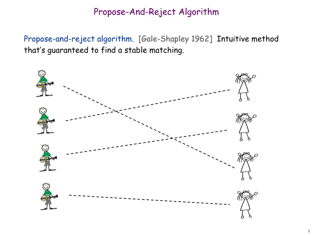
Propose-And-Reject Algorithm Propose-and-reject algorithm. [Gale-Shapley 1962] Intuitive method that s guaranteed to find a stable matching. 1

Stable Matching Problem Perfect matching: everyone is matched monogamously. Each man gets exactly one woman. Each woman gets exactly one man. Stability: no incentive for some pair of participants to undermine assignment by joint action. In matching M, an unmatched pair m-w is unstable if man m and woman w prefer each other to current partners. Unstable pair m-w could each improve by eloping. Stable matching: perfect matching with no unstable pairs. Stable matching problem. Given the preference lists of n men and n women, find a stable matching if one exists. 2

Propose-And-Reject Algorithm Propose-and-reject algorithm. [Gale-Shapley 1962] Intuitive method that guarantees to find a stable matching. Initialize each person to be free. while (some man is free and hasn't proposed to every woman) { Choose such a man m w = 1st woman on m's list to whom m has not yet proposed if (w is free) assign m and w to be engaged else if (w prefers m to her fianc m') assign m and w to be engaged, and m' to be free else w rejects m } 3

Efficient Implementation Efficient implementation. We describe O(n2) time implementation. Representing men and women. Assume men are named 1, , n. Assume women are named 1', , n'. Engagements. Maintain a list of free men, e.g., in a queue. Maintain two arrays wife[m], and husband[w]. set entry to 0 if unmatched if m matched to w then wife[m]=w and husband[w]=m Men proposing. For each man, maintain a list of women, ordered by preference. Maintain an array count[m] that counts the number of proposals made by man m. 4

Efficient Implementation Women rejecting/accepting. Does woman w prefer man m to man m'? For each woman, create inverse of preference list of men. Constant time access for each query after O(n) preprocessing (per woman). 6th 7th 8th 1st 8 2nd 3 3rd 4th 1 5th Amy 5 6 2 Pref 7 4 6 7 8 1 2 3 4 5 Amy 7th 3rd 1st Inverse 4th 8th 2nd 5th 6th Amy prefers man 3 to 6 since inverse[3] < inverse[6] for i = 1 to n inverse[pref[i]] = i 2 7 5

Understanding the Solution Q. For a given problem instance, there may be several stable matchings. Do all executions of Gale-Shapley yield the same stable matching? If so, which one? Def. Man m is a valid partner of woman w if there exists some stable matching in which they are matched. Man-optimal assignment. Each man receives best valid partner. Claim. All executions of GS yield man-optimal assignment, which is a stable matching! No reason a priori to believe that man-optimal assignment is perfect, let alone stable. Simultaneously best for each and every man. 6

Man Optimality Claim. GS matching S* is man-optimal. Pf. (by contradiction) Suppose some man is paired with someone other than best partner. Men propose in decreasing order of preference some man is rejected by valid partner. Let Y be first such man, and let A be first valid woman that rejects him. Let S be a stable matching where A and Y are matched. When Y is rejected, A forms (or reaffirms) engagement with a man, say Z, whom she prefers to Y. Let B be Z's partner in S. Z not rejected by any valid partner at the point when Y is rejected by A. Thus, Z prefers A to B. But A prefers Z to Y. Thus A-Z is unstable in S. S Amy-Yancey Bertha-Zeus . . . since this is first rejection by a valid partner 7

1.2 Five Representative Problems a b b c d e e f g h h T i m e 0 1 2 3 4 5 6 7 8 9 1 1 1 0 A 1 2 1 1 B 2 4 4 5 5 C 3 3 D 4 7 6 6 E 5

Interval Scheduling Input. Set of jobs with start times and finish times. Goal. Find maximum cardinality subset of mutually compatible jobs. jobs don't overlap a b b c d e e f g h h Time 0 1 2 3 4 5 6 7 8 9 10 11 9

Weighted Interval Scheduling Input. Set of jobs with start times, finish times, and weights. Goal. Find maximum weight subset of mutually compatible jobs. 23 12 20 26 13 20 11 16 Time 0 1 2 3 4 5 6 7 8 9 10 11 10

Bipartite Matching Input. Bipartite graph. Goal. Find maximum cardinality matching. A 1 B 2 C 3 D 4 E 5 11

Independent Set Input. Graph. Goal. Find maximum cardinality independent set. subset of nodes such that no two joined by an edge 2 1 1 4 4 5 5 3 7 6 6 12

Competitive Facility Location Input. Graph with weight on each each node. Game. Two competing players alternate in selecting nodes. Not allowed to select a node if any of its neighbors have been selected. Goal. Select a maximum weight subset of nodes. 10 1 5 1 15 1 5 15 5 10 Second player can guarantee 20, but not 25. vs. 13

Five Representative Problems Variations on a theme: independent set. Interval scheduling: n log n greedy algorithm. Weighted interval scheduling: n log n dynamic programming algorithm. Bipartite matching: nk max-flow based algorithm. Independent set: NP-complete. Competitive facility location: PSPACE-complete. 14

Interval Scheduling Input. Set of jobs with start times and finish times. Goal. Find maximum cardinality subset of mutually compatible jobs. jobs don't overlap a b b c d e e f g h h Time 0 1 2 3 4 5 6 7 8 9 10 11 15

Weighted Interval Scheduling Input. Set of jobs with start times, finish times, and weights. Goal. Find maximum weight subset of mutually compatible jobs. 23 12 20 26 13 20 11 16 Time 0 1 2 3 4 5 6 7 8 9 10 11 16

Bipartite Matching Input. Bipartite graph. Goal. Find maximum cardinality matching. A 1 B 2 C 3 D 4 E 5 17

Independent Set Input. Graph. Goal. Find maximum cardinality independent set. subset of nodes such that no two joined by an edge 2 1 1 4 4 5 5 3 7 6 6 18

Competitive Facility Location Input. Graph with weight on each each node. Game. Two competing players alternate in selecting nodes. Not allowed to select a node if any of its neighbors have been selected. Goal. Select a maximum weight subset of nodes. 10 1 5 1 15 1 5 15 5 10 Second player can guarantee 20, but not 25. 19

2.1 Computational Tractability "For me, great algorithms are the poetry of computation. Just like verse, they can be terse, allusive, dense, and even mysterious. But once unlocked, they cast a brilliant new light on some aspect of computing." - Francis Sullivan

Polynomial-Time Brute force. For many non-trivial problems, there is a natural brute force search algorithm that checks every possible solution. Typically takes 2N time or worse for inputs of size N. Unacceptable in practice. n! for stable matching with n men and n women Desirable scaling property. When the input size doubles, the algorithm should only slow down by some constant factor C. There exists constants c > 0 and d > 0 such that on every input of size N, its running time is bounded by cNd steps. Def. An algorithm is poly-time if the above scaling property holds. choose C = 2d 21

Worst-Case Analysis Worst case running time. Obtain bound on largest possible running time of algorithm on input of a given size N. Generally captures efficiency in practice. Draconian view, but hard to find effective alternative. Average case running time. Obtain bound on running time of algorithm on random input as a function of input size N. Hard (or impossible) to accurately model real instances by random distributions. Algorithm tuned for a certain distribution may perform poorly on other inputs. 22

Worst-Case Polynomial-Time Def. An algorithm is efficient if its running time is polynomial. Justification: It really works in practice! Although 6.02 1023 N20 is technically poly-time, it would be useless in practice. In practice, the poly-time algorithms that people develop almost always have low constants and low exponents. Breaking through the exponential barrier of brute force typically exposes some crucial structure of the problem. Exceptions. Some poly-time algorithms do have high constants and/or exponents, and are useless in practice. Some exponential-time (or worse) algorithms are widely used because the worst-case instances seem to be rare. simplex method Unix grep 23

Why It Matters 24

2.2 Asymptotic Order of Growth

Asymptotic Order of Growth Upper bounds. T(n) is O(f(n)) if there exist constants c > 0 and n0 0 such that for all n n0 we have T(n) c f(n). Lower bounds. T(n) is (f(n)) if there exist constants c > 0 and n0 0 such that for all n n0 we have T(n) c f(n). Tight bounds. T(n) is (f(n)) if T(n) is both O(f(n)) and (f(n)). Ex: T(n) = 32n2 + 17n + 32. T(n) is O(n2), O(n3), (n2), (n), and (n2) . T(n) is not O(n), (n3), (n), or (n3). 26

2.4 A Survey of Common Running Times

Linear Time: O(n) Linear time. Running time is at most a constant factor times the size of the input. Computing the maximum. Compute maximum of n numbers a1, , an. max for i = 2 to n { if (ai > max) max } a1 ai 28

Linear Time: O(n) Merge. Combine two sorted lists A = a1,a2, ,an with B = b1,b2, ,bn into sorted whole. i = 1, j = 1 while (both lists are nonempty) { if (ai bj) append ai to output list and increment i else(ai bj)append bj to output list and increment j } append remainder of nonempty list to output list Claim. Merging two lists of size n takes O(n) time. Pf. After each comparison, the length of output list increases by 1. 29

O(n log n) Time O(n log n) time. Arises in divide-and-conquer algorithms. Sorting. Mergesort and heapsort are sorting algorithms that perform O(n log n) comparisons. Largest empty interval. Given n time-stamps x1, , xn on which copies of a file arrive at a server, what is largest interval of time when no copies of the file arrive? O(n log n) solution. Sort the time-stamps. Scan the sorted list in order, identifying the maximum gap between successive time-stamps. 30

Quadratic Time: O(n2) Quadratic time. Enumerate all pairs of elements. Closest pair of points. Given a list of n points in the plane (x1, y1), , (xn, yn), find the pair that is closest. O(n2) solution. Try all pairs of points. min for i = 1 to n { for j = i+1 to n { d (xi - xj)2 + (yi - yj)2 if (d < min) min d } } (x1 - x2)2 + (y1 - y2)2 don't need to take square roots Remark. (n2) seems inevitable, but this is just an illusion. 31

Cubic Time: O(n3) Cubic time. Enumerate all triples of elements. Set disjointness. Given n sets S1, , Sn each of which is a subset of 1, 2, , n, is there some pair of these which are disjoint? O(n3) solution. For each pairs of sets, determine if they are disjoint. foreach set Si { foreach other set Sj { foreach element p of Si { determine whether p also belongs to Sj } if (no element of Si belongs to Sj) report that Si and Sj are disjoint } } 32

Polynomial Time: O(nk) Time Independent set of size k. Given a graph, are there k nodes such that no two are joined by an edge? k is a constant O(nk) solution. Enumerate all subsets of k nodes. foreach subset S of k nodes { check whether S in an independent set if (S is an independent set) report S is an independent set } } Check whether S is an independent set = O(k2). Number of k element subsets = O(k2 nk / k!) = O(nk). nk n k =n (n 1) (n 2) k (k 1) (k 2) (n k+1) (2) (1) k! poly-time for k=17, but not practical 33

Exponential Time Independent set. Given a graph, what is maximum size of an independent set? O(n2 2n) solution. Enumerate all subsets. S* foreach subset S of nodes { check whether S in an independent set if (S is largest independent set seen so far) update S* S } } 34

The Plan for the rest of the quarter See some algorithms. Divide and conquer, greedy, dynamic programming. NP-completeness. Some problems are so hard, we don t think they have any polynomial-time algorithm. Reductions. A lot of these problems (literally thousands), coming from every area of science, engineering, technology, industry, medicine, are really the same problem in disguise. More: CSE 421 Algorithms (Winter, Rao) CSE 431 Complexity (Spring, Lee) CSE 446 Machine Learning (Winter, Etzioni) 35