Heuristic Approach and Simulated Annealing: Optimization Strategies

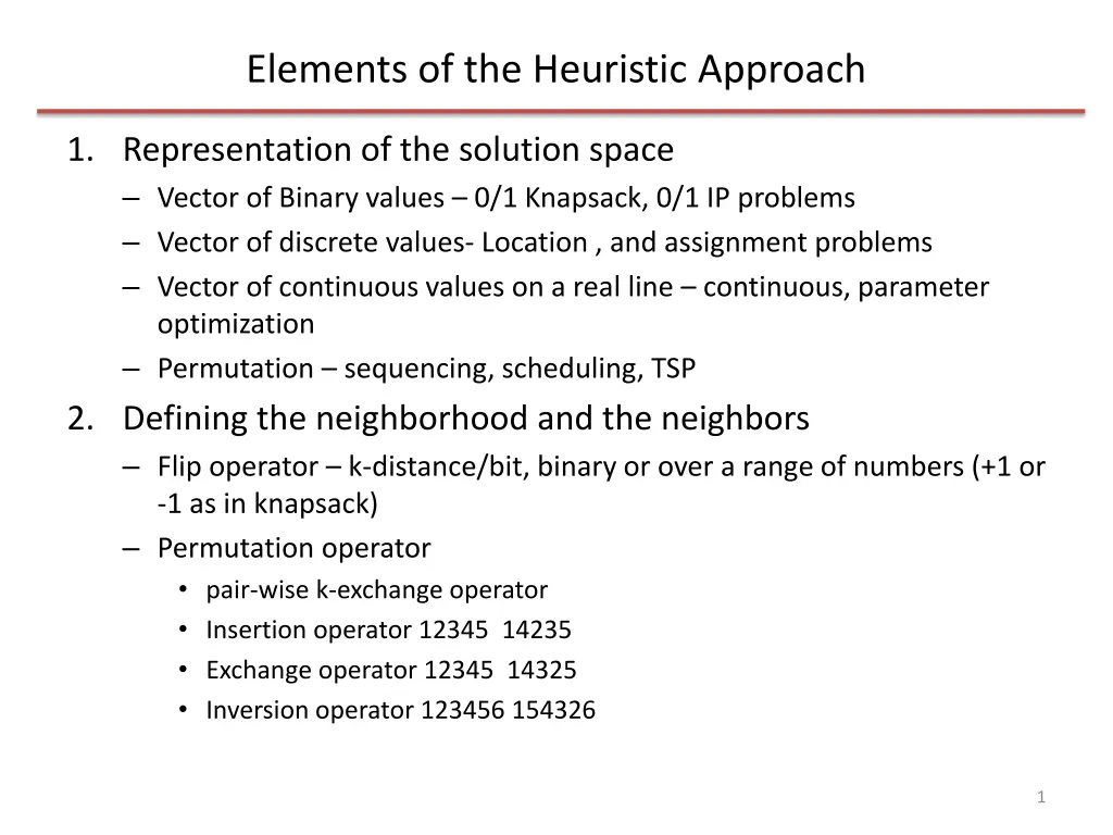
Elements of the Heuristic Approach 1. Representation of the solution space Vector of Binary values 0/1 Knapsack, 0/1 IP problems Vector of discrete values- Location , and assignment problems Vector of continuous values on a real line continuous, parameter optimization Permutation sequencing, scheduling, TSP 2. Defining the neighborhood and the neighbors Flip operator k-distance/bit, binary or over a range of numbers (+1 or -1 as in knapsack) Permutation operator pair-wise k-exchange operator Insertion operator 12345 14235 Exchange operator 12345 14325 Inversion operator 123456 154326 1

Elements of the Heuristic Approach 3. Defining the initial solution Random or greedy 4. Choosing the method (algorithm for iterative search) Off-the shelf or tailor made heuristic Single-start or multistart (still single but several independent singles) or population (solutions interact with one another) Strategies for escaping local optima Balance diversification and intensification of search 5. Objective function evaluation Full or partial evaluation At every iteration or after a set of iterations 6. Stopping criteria Number of iterations Time Counting the number of non-improving solutions in consecutive iterations. Remember: there is a lot of flexibility in setting up the above. Optimality cannot be proved. All you are looking for is a good solution given the resource (time, money and computing power) constraints 2

Escaping local optimas Accept nonimproving neighbors Tabu search and simulated annealing Iterating with different initial solutions Multistart local search, greedy randomized adaptive search procedure (GRASP), iterative local search Changing the neighborhood Variable neighborhood search Changing the objective function or the input to the problem in a effort to solve the original problem more effectively. Guided local search 3

Simulated Annealing Based on material science and physics Annealing: For structural strength of objects made from iron, annealing is a process of heating and then slow cooling to form a strong crystalline structure. The strength depends on the cooling rate If the initial temperature is not sufficiently high or the cooling is too fast then imperfections are obtained SA is an analogous process to the annealing process 4

SA The objective of SA is to escape local optima and to delay convergence. SA is a memoryless heuristic approach Start with an initial solution At each iteration obtain a neighbor in a random or organized way Moves that improve the solution are always accepted Moves that do not improve the solution are accepted using a probability. By the law of thermodynamics at temperature t, the probability of an increase in energy of magnitude E is given by P( E,t)= exp(- E/kt) Where k is the Boltzmann s constant For min problems E = f(current move)-f(last move) For max problem E = f(lastmove)- f(current move) Keep E positive 5

SA The acceptance probability of a non-improving solution is P( E,t) > R Where R is a uniform random number between 0 and 1 Sometimes R can be fixed at 0.5 At a given temperature many trials can be explored As the temperature cools the acceptance probability of a non- improving solution decreases. In solving optimization problems let kt = T P( E,t)= exp(- E/kt) In summary, other than the standard design parameters such as neighborhood and initial solution, the two main design parameters are Cooling schedule Acceptance probability of non-improving solutions which depends on the initial temperature 6

SA acceptance probability of non-improving solutions At high temperature, the acceptance probability is high When T = all moves are accepted When T ~ 0 no non-improving moves are accepted Note the above decrease in accepting non-improving moves is exponential. Setting initial temperature Set very high accept all moves- high computation cost Using standard deviation of the difference between objective function values obtained from preliminary experimentation. T= c c= -3/ln(p) p= acceptance probability 7

SA Cooling schedules Linear Ti= T0 i where i is the iteration number and is a constant Geometric Ti= Ti-1 where is a constant, 0< <1 Logarithmic Ti= T0/ln(i) The cooling rate is very slow but can help to reach global optimum. Computationally intensive Nonmonotonic Temp is increased again during the search to encourage diversification. Adaptive Dynamic cooling schedule. Adjust based on characteristics of the search landscape A large number of iterations at low temp (follow Logarithmic) and a small number of iterations at high temp (follow Geometric) 8

SA stopping criteria Reaching the final temperature Achieving a pre-determined number of iterations Keeping a counter on the number of times a certain percentage of neighbors at each temperature is accepted. Examples 9