High-Resolution Climate Modelling Requirements from ECVs
Climate modelling project PRIMAVERA aims to deliver innovative high-resolution global climate models to improve regional climate projections. The project focuses on understanding important weather and climate processes at sub-50km resolution, exploring global drivers of climate variability, and assessing impacts on regional climate. Through coordinated experimental design and model integrations, PRIMAVERA seeks to enhance our knowledge of climate processes and provide actionable climate information for societal risk management.

Download Presentation

Please find below an Image/Link to download the presentation.
The content on the website is provided AS IS for your information and personal use only. It may not be sold, licensed, or shared on other websites without obtaining consent from the author.If you encounter any issues during the download, it is possible that the publisher has removed the file from their server.
You are allowed to download the files provided on this website for personal or commercial use, subject to the condition that they are used lawfully. All files are the property of their respective owners.
The content on the website is provided AS IS for your information and personal use only. It may not be sold, licensed, or shared on other websites without obtaining consent from the author.
E N D
Presentation Transcript
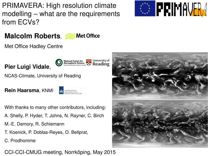
PRIMAVERA: High resolution climate modelling what are the requirements from ECVs? Malcolm Roberts, Met Office Hadley Centre Pier Luigi Vidale, NCAS-Climate, University of Reading Rein Haarsma, KNMI With thanks to many other contributors, including: A. Shelly, P. Hyder, T. Johns, N. Rayner, C. Birch M.-E. Demory, R. Schiemann T. Koenick, P. Doblas-Reyes, O. Bellprat, C. Prodhomme CCI-CCI-CMUG meeting, Norrk ping, May 2015
Talk outline Overview of H2020 PRIMAVERA and CMIP6 HighResMIP Examples of science questions Requirements of ECVs Examples of how ECVs are or could be used Some initial Met Office work with CCI SST
Malcolm Roberts, Met Office (coordinator) Pier Luigi Vidale, Univ. of Reading (scientific coordinator) PRocess-based climate sIMulation: AdVances in high resolution modelling and European climate Risk Assessment Goal: to deliver novel, advanced and well-evaluated high-resolution global climate models (GCMs), capable of simulating and projecting regional climate with unprecedented fidelity, out to 2050. To deliver: innovative climate science and a new generation of European advanced GCMs. improve understanding of the drivers of variability and change in European climate, including extremes, which continue to be characterised by high uncertainty new climate information that is tailored, actionable and strengthens societal risk management decisions with sector-specific end-users new insights into climate processes using eddy-resolving ocean and explicit convection atmosphere models To run for 4 years from Nov 2015 including 19 partners across Europe, funded by the Horizon 2020 call SC5-1-2014 - Advanced Earth System Models proj.badc.rl.ac.uk/primavera Core integrations in PRIMAVERA will form much of the European contribution to CMIP6 HighResMIP http://www.wcrp-climate.org/index.php/modelling-wgcm-mip-catalogue/429-wgcm-hiresmip
Rein Haarsma KNMI (lead) Malcolm Roberts Met Office (co-lead) CMIP6 HighResMIP Important weather and climate processes emerge at sub-50km resolution They contribute significantly to both large-scale circulation and local impacts, hence vital for understanding and constraining regional variability How robust are these effects? Is there any convergence with resolution across models? Need coordinated, simplified experimental design to find out http://www.wcrp-climate.org/index.php/modelling-wgcm-mip- catalogue/429-wgcm-hiresmip Global drivers Regional variability Feedbacks to large scale Experimental protocol: Global models AMIP-style and coupled Physical climate system only Integrations: 1950-2050 Ensemble size: >=1 (ideally 3) Resolutions: <25km HI and ~60-100km STD Aerosol concentrations specified Local processes Impacts, extremes e.g. Zhao et al, 2009; Haarsma et al, 2013; Demory et al, 2013
HighResMIP and PRIMAVERA Horizon 2020 PRIMAVERA European focus Model assessment Model development Frontier simulations Drivers of clim var Inform climate risk CMIP6 HighResMIP International community Multi-model global high & std resolution climate simulations Main European contribution to HighResMIP Resolution is our chosen tool for investigation and understanding Ensembles, complexity, parameter uncertainty and initialisation are other axes All need suitable datasets for assessment
Aim: to discover at what resolution climate processes are robustly simulated across Example map of climate process and model resolution required Joint Weather and Climate Research Programme A partnership in climate research multi-model ensemble
HighResMIP pushing the boundaries of CMIP Detailed model process evaluation Moving away from using monthly means and climatologies towards high frequency interactions and extreme processes Requires much more detail from observations and reanalyses Requirements for simulations: High resolution, daily SST and sea-ice forcing (cf monthly mean, ~1 ) High frequency output 6hr, 3hr and 1hr diagnostics, particularly for extreme processes (precipitation, cyclones) and interactions (e.g. air-sea, land- atmosphere) Longer integrations of AMIP-style forced-atmosphere to sample phases of climate modes such as AMO, PDO and their teleconnections 14 international groups have committed to AMIP-style HighResMIP simulations (1950-2050) at both a standard (~100km) and a high resolution (~25km) Opportunity for modelling and observational communities since we are studying similar space and timescales
European HighResMIP resolutions (as part of PRIMAVERA) Institution MO NCAS KNMI IC3 SMHI CNR ECEarth NEMO T255-799 CERFACS MPI AWI CMCC ECMWF Model namesMetUM ECHAM FESOM T63-255 Arpege NEMO T127-359 ECHAM MPIOM T63-255 CCESM NEMO 100-25km IFS NEMO T319-799 NEMO 60-25km Atmosph. Res., core Oceanic Res., core o o 0.4- o 1- spatially variable 1/10 Spatially variable Oceanic Res., Frontiers 1/12 1/12 1/10 Concentrate on horizontal resolution keep vertical resolution the same Global atmosphere resolutions: range from 150km to 6km Global ocean resolutions: from 1 to 1/12
PRIMAVERA themes and work packages
PRIMAVERA work areas European climate process focus Development of metrics for model assessment Work on UK Auto-assess package Plan to merge with ESMValTool later in 2016 Requirements Assess impact of model resolution, model physics and sub-grid scale processes (parameterisations) Range of timescales hours to decades Focus on variability and extremes Use them to understand and constrain spread in climate projections (interactions between processes) Provide policy-relevant climate information
Process understanding Precipitation and energy Precip over land, sea, orography Using models to try and interpret observations, constraints Understand whether model or observational biases Demory-ogram hydrological cycle, tying together energy and water Air sea interactions Models typically have weaker coupling than observed Possibly relates to weak signal to noise e.g. Large ensembles required Need co-located SST, wind, flux, moisture in order to understand interactions, at high frequency Diurnal cycle Cloud, soil moisture, water vapour, temperature, precipitation
Constraining the global energy and water budgets and transport How well do models compare with observations Can observations rule out any models Models are energetically consistent unlike different observational datasets Can models help to understand and constrain observations Transport of water and its change (either via variability or global warming) key for impacts What impact does horizontal resolution have Want models to be able to represent correct budgets and transports To give confidence in any changes they may project Changes will be much smaller than means challenging problem
What does not change with resolution? The global energy budget Wild et al, 2012 Equivalent estimates in Stephens et al, 2012 Resolution at 50N: 270 km 135 km 90 km 60 km 40 km 25 km Demory et al., Clim. Dyn., 2014 Figure adapted from Trenberth et al, 2009 Fluxes: W/m2
What does change with resolution? The global hydrological cycle Classic GCMs too dependent on physical parameterisation because of unresolved atmospheric transports Role of resolved sea->land transport larger at high resolution Hydrological cycle more intense at high resolution Resolution at 50N: 270 km 135 km 90 km 60 km 40 km 25 km Demory et al., Clim. Dyn., 2014 Figure adapted from Trenberth et al, 2007, 2011
Relative roles of remote transport and local re- cycling in forming precipitation over land Transport of water from ocean to land Local recycling of precipitation For this aspect of the simulation of the Global Climate system, models are converging and we know what resolution is adequate. Resolution High local recycling Low transport Lower local recycling Higher transport Demory et al, Clim. Dyn., 2014
Understanding causes of hydrological changes with model resolution ocean-to-land water transport and global land precipitation has been shown to increase with AGCM resolution (Demory et al., 2014) 1. What is the role of better resolved orography at higher model resolution? 2. How well is the amount of land precipitation (spatial averages over large areas) constrained by observations?
Global mean Schiemann et al., in prep
Example: Europe JJA DJF Schiemann et al., in prep
SST-wind speed relationships at monthly and daily timescales Monthly mean SST/wind speed regression Daily SST/wind speed regression ORCA 1/4 ORCA 1/4 ORCA 1/12 ORCA 1/12 Courtesy Ann Shelly
SST-wind stress coupling strength N512-ORCA12 N216-ORCA025 OBS (Jan-Feb for AGUL and GS, 2003-2007 for KUR) 0.016 0.006 0.017 0.011 0.005 0.014 0.007 0.006 0.01 0.026 0.011 0.015 0.007 0.007 0.002 0.01 Courtesy Ann Shelly
Regression between monthly SST anomaly and monthly net heat flux anomaly Different model resolutions Observations = Reynolds OI SST and fluxes derived from TOA and ERAI (Liu et al, submitted)
Localtime of peak precipitation for 12km models (diurnal cycle) Jan-Dec 2006 Joint Weather and Climate Research Programme A partnership in climate research Birch et al, in revision
ECV properties Global coverage Long time period, homogeneous datasets Gridded, quality controlled, familiar data formats Quantified uncertainties Easily searchable, downloadable Co-location of related quantities for understanding processes Availability of multiple observations of same ECV for comparison, understanding uncertainty
Precipitation and orography 3hr precipitation for diurnal cycle Rainfall over steep orography reduced biases Ocean Sub-daily SST product to assess diurnal cycle In-situ heat fluxes over ocean Including temperature, humidity, wind in order to validate turbulent fluxes and parameterisations in models
Clouds and aerosols Cloud properties big differences in observational estimates Droplet number Effective size Ice water path Lightning Satellites detect light mainly cloud to cloud Radio detect mainly cloud to ground Models simulate both how to assess Differentiation between cloud regimes/different cloud layers Estimates of vertical velocity would be amazing to look at convective up and downdrafts
Sea-ice Volume the combination of snow and sea ice Closely related to energy budget, and hence essential to understand and constrain model processes (and for understanding global warming) Thickness Albedo (particularly over sea-ice) constrain parameterisations Understand feedbacks, climate sensitivity Short length of series - 1992-2008 for ice concentration, few years for thickness Quality problems sea-ice detected far from ice edge (being worked on)
Land surface Soil moisture Dataset produced confined to surface Really want down to root zone, ~2m To use in models to understand vegetation dynamics, need to create model+data hybrid to produce a type of soil moisture that we can use to understand vegetation dynamics Standardising such hybrid methods is important Indicator of vegetation activity, e.g. fPAR Fraction of Absorbed Photosynthetically Active Radiation This biophysical variable is directly related to the primary productivity of photosynthesis and some models use it to estimate the assimilation of carbon dioxide in vegetation. use to estimate whether or not vegetation is stressed (soil moisture stress and/or temperature stress). Water table depth Enable understanding of global transports of water
Initial Met Office work using CCI SST Several 25km integrations complete using CCI SST and sea-ice as driving data (together with 130km simulations for comparison) To compare with standard model development integrations using Reynolds OI
Comparing different SST datasets over long timescales
Precipitation change: Model resolution vs SST forcing Impact of model resolution Impact of SST forcing at same resolution JJA precip: 25km 130km simulation, 18yr mean JJA precip: 25km: CCI Reynolds OI 18yr mean 25km model bias vs GPCP2
Changes in tropical cyclone climatology with different SST forcings Daily Reynolds OI Daily CCI Monthly HadISST Rey CCI HadISST Obs
Future plans Testing and understanding impact of using different forcing datasets on model simulations Differences between ECVs is much smaller than coupled model biases However can still have a significant effect on other quantities of interest Understanding relative impact of Uncertainty in ECVs (running ensembles of models with different forcing/including uncertainty) Quantifying impact of these uncertainties on response of relevant climate variables and processes Make use of CCI datasets in PRIMAVERA work packages Metrics Model development and assessment both core and frontier simulations
UPSCALE: UK on PRACE - weather resolving Simulations of Climate for globAL Environmental risk PI: P.L. Vidale, NCAS-Climate, Reading Joint Weather and Climate Research Programme A partnership in climate research AIM: To increase understanding of climate processes and their resolution dependence Forced atmosphere-land integrations, 1985-2011, 3-5 ensemble members/resolution SST and sea-ice forcing from OSTIA 1/20 daily data CMIP5-defined forcings including historic aerosol emissions Timeslice future climate for 2100 with SST from HadGEM2-ES using RCP8.5, 3 ensemble members/resolution Using PRACE HPC grant of 144M core hours on HLRS Stuttgart CRAY XE6 400TB data produced Demory et al (2013), Mizielinski et al (2014), Allan et al 2014, Roberts et al 2015, Vidale et al (in prep), Bush et al (in revision), Vellinga et al (in revision) 500 1500 orography (m) UPSCALE: HadGEM3-A GA3.0 (85 levels, top@85km) Essentially the same physics/dynamics parameters used throughout model hierarchy 5 members 3 members 5 members N512 (25 km) N216 (60 km) N96 (135 km) Resolution increase
UK HighResMIP - PRIMAVERA UK results Impact of resolution and links to multiple model biases e.g. Sahel rainfall and decadal variability, AEJ/AEWs, Atlantic tropical cyclones Eddy resolving ocean, improved ocean circulation, reduced Southern Ocean biases, improved Atlantic Individual or small group campaigns E.g. Athena, UPSCALE, HiResCLIM, EC-Earth, STORM, Climate-SPHINX Leading to HighResMIP Coordinated international multi-model high resolution comparison Robustness across multi-models Leading to PRIMAVERA Model development and assessment with focus on Europe Frontier simulations
Modelling groups expressing interest in HighResMIP (at least for Tier 1 simulations) Group Country Model China BCC BCC-CSM2-HR Brazil INPE BESM China Chinese Academy of Meteorological Sciences CAMS-CSM China Institute of Atmospheric Physics, Chinese Academy of Sciences FGOALS USA NCAR CESM China Center for Earth System Science/Tsinghua University CESS/THU Italy Centro Euro-Mediterraneo sui Cambiamenti Climatici CMCC France CNRM-CERFACS CNRM Europe EC-Earth consortium (11 groups) EC-Earth USA GFDL GFDL Russia Institute of Numerical Mathematics INM Japan AORI, University of Tokyo / JAMSTEC / National Institute for Environmental Studies MIROC6-CGCM Japan AORI, University of Tokyo / JAMSTEC / National Institute for Environmental Studies NICAM Germany Max Planck Institute for Meteorology (MPI-M) MPI-ESM Japan Meteorological Research Institute MRI-AGCM3.xS UK Met Office UKESM /HadGEM3
Global HighResMIP resolution representation of orography 130km resolution orography Illustration of the orographic representation at standard and high resolution over Europe in a global model. Orographic processes are highly non-linear 25km resolution orography
High resolution climate modelling - multi-resolution and multi-model robustness Need a traceable resolution hierarchy with no tuning between resolutions UPSCALE tropical cyclones, moisture transports, tropical precipitation explicit convection diurnal cycle, land-atmosphere interaction, precipitation intensity ORCA12 mean state, air-sea interaction Towards multi-model robust changes with resolution alone (no resolution-specific tuning) Give examples of these from UK group, what answers and questions there are and how multi-model can help to address these CMIP5/IPCC AR5 questions
MetUM global atmosphere/coupled model climate configurations in use Atmosphere/land GloSea5 UPSCALE N216 N512 60km 25km N144 N768 90km 17km N96 UK-ESM1 for CMIP6? N1024 130km ORCA025 12km 0.25 ORCA12 ORCA1 0.08 1 Explicit convection Ocean/sea-ice Charisma project Project to assess impact of global explicit convection CMIP3&CMIP5 resolution Essentially the same physics/dynamics parameters used throughout model hierarchy GA = Global Atmosphere GC = Global Coupled


")
")