Identified Transfer Function Models and System Response Comparison
Learn how transfer function models were estimated and system responses compared using hand calculations in Matlab System Identification. See visual representations of the fitted DCP models and the discrepancy between the hand-derived DCP model response and simulated outputs.

Download Presentation

Please find below an Image/Link to download the presentation.
The content on the website is provided AS IS for your information and personal use only. It may not be sold, licensed, or shared on other websites without obtaining consent from the author. If you encounter any issues during the download, it is possible that the publisher has removed the file from their server.
You are allowed to download the files provided on this website for personal or commercial use, subject to the condition that they are used lawfully. All files are the property of their respective owners.
The content on the website is provided AS IS for your information and personal use only. It may not be sold, licensed, or shared on other websites without obtaining consent from the author.
E N D
Presentation Transcript
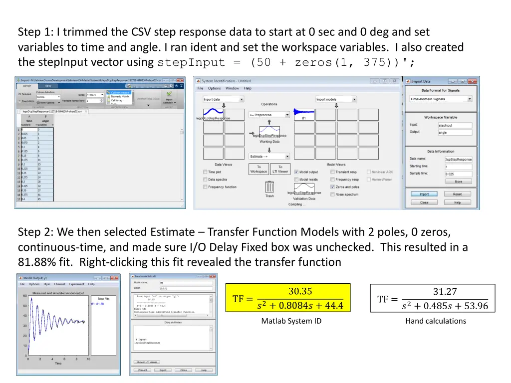
Step 1: I trimmed the CSV step response data to start at 0 sec and 0 deg and set variables to time and angle. I ran ident and set the workspace variables. I also created the stepInput vector using stepInput = (50 + zeros(1, 375))'; Step 2: We then selected Estimate Transfer Function Models with 2 poles, 0 zeros, continuous-time, and made sure I/O Delay Fixed box was unchecked. This resulted in a 81.88% fit. Right-clicking this fit revealed the transfer function 30.35 31.27 TF = TF = ?2+ 0.8084? + 44.4 ?2+ 0.485? + 53.96 Matlab System ID Hand calculations
Step 3: Matlab System ID called fit tf1. Used pole(tf1) to determine poles 30.35 31.27 TF = TF = ?2+ 0.8084? + 44.4 ?2+ 0.485? + 53.96 Hand calculations Matlab System ID Poles = 0.4042 6.6511? Poles = 0.2425 7.3417? ? = tan 10.4042 ? = tan 10.2425 6.6511= 0.061 deg 7.3417= 0.033 deg ? = sin0.061 = ?.??? ? = sin0.033 = ?.??? 0.40422+ 6.65112= 0.24252+ 7.34172= ??= 0.1634 + 44.23 = 44.40 = ?.?? ??= 0.059 + 53.9 = 53.96 = ?.??
Scope output for fitted DCP model simulinkDcpStepInputFittedModel112818a.slx 11/12/18 Evernote results i.e. hand-derived DCP model response. Compared to figure on the left, this model doesn t match as well Overlay of CSV file (red) on simulated output
simulinkDcpPidFittedModel112818a.slx Scope output for fitted DCP model with PID 10/26/18 Evernote results i.e. hand-derived DCP model response Not too much difference Overlay of CSV file (red) on simulated output
00courses\...\labview-XX-MatlabSystemId\legoDcpPolePlacementGains1_0.m00courses\...\labview-XX-MatlabSystemId\legoDcpPolePlacementGains1_0.m Scope output for fitted DCP model with PID FILE: legoDcpPolePlacementFittedModel1_0.slx

 to")


