IEEE 802.15 TG6ma January 2023 Closing Report
This document contains the closing report for TG15.6ma in January 2023, focusing on the revision of IEEE P802.15.6-2012 with enhanced dependability. The report includes objectives, actions taken, session schedules, and details of the interim session in Baltimore, USA.

Download Presentation

Please find below an Image/Link to download the presentation.
The content on the website is provided AS IS for your information and personal use only. It may not be sold, licensed, or shared on other websites without obtaining consent from the author.If you encounter any issues during the download, it is possible that the publisher has removed the file from their server.
You are allowed to download the files provided on this website for personal or commercial use, subject to the condition that they are used lawfully. All files are the property of their respective owners.
The content on the website is provided AS IS for your information and personal use only. It may not be sold, licensed, or shared on other websites without obtaining consent from the author.
E N D
Presentation Transcript
Environmental Data Analysis with MATLAB or Python 3rdEdition Lecture 20
SYLLABUS Lecture 01 Lecture 02 Lecture 03 Lecture 04 Lecture 05 Lecture 06 Lecture 07 Lecture 08 Lecture 09 Lecture 10 Lecture 11 Lecture 12 Lecture 13 Lecture 14 Lecture 15 Lecture 16 Lecture 17 Lecture 18 Lecture 19 Lecture 20 Lecture 21 Lecture 22 Lecture 23 Lecture 24 Lecture 25 Lecture 26 Intro; Using MTLAB or Python Looking At Data Probability and Measurement Error Multivariate Distributions Linear Models The Principle of Least Squares Prior Information Solving Generalized Least Squares Problems Fourier Series Complex Fourier Series Lessons Learned from the Fourier Transform Power Spectra Filter Theory Applications of Filters Factor Analysis and Cluster Analysis Empirical Orthogonal functions and Clusters Covariance and Autocorrelation Cross-correlation Smoothing, Correlation and Spectra Coherence; Tapering and Spectral Analysis Interpolation and Gaussian Process Regression Linear Approximations and Non Linear Least Squares Adaptable Approximations with Neural Networks Hypothesis testing Hypothesis Testing continued; F-Tests Confidence Limits of Spectra, Bootstraps
Goals of the lecture Part 1 Finish up the discussion of correlations between time series Part 2 Examine how the finite observation time affects estimates of the power spectral density of time series
Part 1 Coherence frequency-dependent correlations between time series
Scenario A in a hypothetical region windiness and temperature correlate at periods of a year, because of large scale climate patterns but they do not correlate at periods of a few days
wind speed 1 2 3 time, years temperature 1 2 3 time, years
summer hot and windy winters cool and calm wind speed 1 2 3 time, years temperature 1 2 3 time, years
heat wave not especially windy cold snap not especially calm wind speed 1 2 3 time, years temperature 1 2 3 time, years
in this case times series correlated at long periods but not at short periods
Scenario B in a hypothetical region plankton growth rate and precipitation correlate at periods of a few weeks but they do not correlate seasonally
growth rate 1 2 3 time, years precipitation 1 2 3 time, years
growth rate has no seasonal signal plant growth rate summer drier than winter 1 2 3 time, years precipitation 1 2 3 time, years
growth rate high at times of peak precipitation plant growth rate 1 2 3 time, years precipitation 1 2 3 time, years
in this case times series correlated at short periods but not at long periods
Coherence a way to quantify frequency-dependent correlation
strategy band pass filter the two time series, u(t) and v(t) around frequency, 0 compute their zero-lag cross correlation (large when time series are similar in shape) repeat for many 0 s to create a function c( 0)
band pass filter f(t) has this p.s.d. |f( )|2 2 2 - 0 0 0
evaluate at zero lag t=0 and at many 0 s
Short Cut Fact 1 A function evaluates at time t=0 is equal to the integral of its Fourier Transform Fact 2 the Fourier Transform of a convolution is the product of the transforms
integral over frequency assume ideal band pass filter that is either 0 or 1 negative frequencies positive frequencies
integral over frequency assume ideal band pass filter that is either 0 or 1 negative frequencies positive frequencies c is real so real part is symmetric, adds imag part is antisymmetric, cancels
integral over frequency assume ideal band pass filter that is either 0 or 1 negative frequencies positive frequencies c is real so real part is symmetric, adds imag part is antisymmetric, cancels interpret intergral as an average over frequency band
integral over frequency can be viewed as an average over frequency (indicated with the overbar)
Two final steps 1. Omit taking of real part in formula (simplifying approximation) 2. Normalize by the amplitude of the two time series and square, so that result varies between 0 and 1
the final result is called Coherence
precipitation A) 5 0 0 200 400 600 800 1000 1200 1400 1600 B) new dataset: 20 T-air 10 0 0 200 400 600 800 1000 1200 1400 1600 C) Water Quality 20 T-water 10 0 0 200 400 600 800 1000 1200 1400 1600 D) Reynolds Channel, Coastal Long Island, New York 34 salinity 32 30 28 0 200 400 600 800 time, days 1000 1200 1400 1600 E) turbidity 20 0 0 200 400 600 800 time, days 1000 1200 1400 1600 F) chlorophyll 20 0 0 200 400 600 800 time, days 1000 1200 1400 1600
precipitation precipitation A) 5 0 0 200 400 600 800 1000 1200 1400 1600 air temperature B) new dataset: 20 T-air 10 0 0 200 400 600 800 1000 1200 1400 1600 water temperature C) Water Quality 20 T-water 10 0 0 200 400 600 800 1000 1200 1400 1600 D) Reynolds Channel, Coastal Long Island, New York salinity 34 salinity 32 30 28 0 200 400 600 800 time, days 1000 1200 1400 1600 E) turbidity turbidity 20 0 0 200 400 600 800 time, days 1000 1200 1400 1600 F) chlorophyl chlorophyll 20 0 0 200 400 600 800 time, days 1000 1200 1400 1600
A) periods near 1 year B) periods near 5 days 1 0.05 precip 0 precip 0 -1 -0.05 -2 400 450 500 550 0 200 400 600 800 1000 1200 1400 1600 4 10 2 T-air T-air 0 0 -2 -4 -10 400 450 500 550 0 200 400 600 800 1000 1200 1400 1600 10 1 T-water T-water 0 0 -1 -10 400 450 500 550 0 200 400 600 800 1000 1200 1400 1600 0.6 10 0.4 salinity salinity 0.2 0 -0.20 -0.4 -10 400 450 500 550 0 200 400 600 800 time, days 1000 1200 1400 1600 time, days 2 -101 turbidity turbidity 0 -2 -2 -4 -3 400 450 500 550 0 200 400 600 800 time, days 1000 1200 1400 1600 time, days -2024 2 chlorophyl chlorophyl 0 -4 -2 -6 400 450 500 550 0 200 400 600 800 time, days 1000 1200 1400 1600 time, days Fig, 9.18. Band-pass filtered water quality measurements from Reynolds Channel (New York) for several years starting January 1, 2006. A) Periods near one year; and B) periods near 5 days. MatLab script eda09_16.
A) periods near 1 year B) periods near 5 days 1 0.05 precip 0 precip 0 -1 -0.05 -2 400 450 500 550 0 200 400 600 800 1000 1200 1400 1600 4 10 2 T-air T-air 0 0 -2 -4 -10 400 450 500 550 0 200 400 600 800 1000 1200 1400 1600 10 1 T-water T-water 0 0 -1 -10 400 450 500 550 0 200 400 600 800 1000 1200 1400 1600 0.6 10 0.4 salinity salinity 0.2 0 -0.20 -0.4 -10 400 450 500 550 0 200 400 600 800 time, days 1000 1200 1400 1600 time, days 2 -101 turbidity turbidity 0 -2 -2 -4 -3 400 450 500 550 0 200 400 600 800 time, days 1000 1200 1400 1600 time, days -2024 2 chlorophyl chlorophyl 0 -4 -2 -6 400 450 500 550 0 200 400 600 800 time, days 1000 1200 1400 1600 time, days Fig, 9.18. Band-pass filtered water quality measurements from Reynolds Channel (New York) for several years starting January 1, 2006. A) Periods near one year; and B) periods near 5 days. MatLab script eda09_16.
B) C) A) precipitation and salinity air-temp and water-temp water-temp and chlorophyll 1 1 1 one year coherence coherence coherence 0.5 0.5 0.5 one year one week 0 0 0 0 0.05 0.1 0.15 0.2 0 0.05 0.1 0.15 0.2 0 0.05 0.1 0.15 0.2 frequency, cycles per day frequency, cycles per day frequency, cycles per day
high coherence at periods of 1 year B) C) A) precipitation and salinity air-temp and water-temp water-temp and chlorophyll 1 1 1 one year coherence coherence coherence 0.5 0.5 0.5 one year one week 0 0 0 0 0.05 0.1 0.15 0.2 0 0.05 0.1 0.15 0.2 0 0.05 0.1 0.15 0.2 frequency, cycles per day frequency, cycles per day frequency, cycles per day moderate coherence at periods of about a month very low coherence at periods of months to a few days
Part 2 windowing time series before computing power- spectral density
1 10 ASD of d d(t) 0 5 scenario: you are studying an indefinitely long phenomenon -1 0 0 200 time t, s 400 0 0.1 0.2 0.3 0.4 frequency f, Hz 1 10 1 ASD of d ASD of W d(t) 0 5 5 W(t) 0 -1 0 -1 0 0 200 time t, s 400 0 0.1 0.2 0.3 0.4 0 200 time t, s 400 0 0.1 0.2 0.3 0.4 frequency f, Hz frequency f, Hz but you only observe a short portion of it 1 1 4 5 ASD of W ASD of Wd) W(t)*d(t) W(t) 0 0 2 -1 0 -1 0 0 200 time t, s 400 0 0.1 0.2 0.3 0.4 0 200 time t, s 400 0 0.1 0.2 0.3 0.4 frequency f, Hz frequency f, Hz 1 4 ASD of Wd) W(t)*d(t) 0 2 -1 0 0 200 time t, s 400 0 0.1 0.2 0.3 0.4 frequency f, Hz
how does the power spectral density of the short piece differ from the p.s.d. of the indefinitely long phenomenon (assuming stationary time series)
1 10 ASD of d d(t) 0 5 -1 0 0 200 time t, s 400 0 0.1 0.2 0.3 0.4 frequency f, Hz 1 1 1 10 10 ASD of d ASD of d ASD of W 5 5 5 d(t) d(t) 0 0 W(t) 0 -1 -1 0 0 -1 0 0 200 time t, s time t, s 400 400 0 0 0.1 0.1 0.2 0.2 0.3 0.3 0.4 0.4 0 200 0 200 time t, s 400 0 0.1 0.2 0.3 0.4 We might suspect that the difference will be increasingly significant as frequency f, Hz frequency f, Hz frequency f, Hz 1 1 1 4 5 5 ASD of W the window of observation ASD of Wd) becomes so short that it includes just a few oscillations of the period of interest. 2 ASD of W W(t)*d(t) W(t) 0 W(t) 0 0 2 -1 0 -1 -1 0 0 0 200 time t, s 400 0 0.1 0.2 0.3 0.4 0 0 200 400 400 0 0 0.1 0.1 0.2 0.2 0.3 0.3 0.4 0.4 200 time t, s time t, s frequency f, Hz frequency f, Hz frequency f, Hz 1 4 4 1 ASD of Wd) ASD of Wd) W(t)*d(t) W(t)*d(t) 0 2 0 -1 -1 0 0 0 200 time t, s time t, s 400 400 0 0 0.1 0.1 0.2 0.2 0.3 0.3 0.4 0.4 0 200 frequency f, Hz frequency f, Hz
starting point short piece is the indefinitely long time series multiplied by a window function, W(t)
1 10 ASD of d d(t) 0 5 -1 0 0 200 time t, s 400 0 0.1 0.2 0.3 0.4 frequency f, Hz 1 ASD of W 5 W(t) 0 -1 0 0 200 time t, s 400 0 0.1 0.2 0.3 0.4 frequency f, Hz 1 4 ASD of Wd) W(t)*d(t) 0 2 -1 0 0 200 time t, s 400 0 0.1 0.2 0.3 0.4 frequency f, Hz
by the convolution theorem Fourier Transform of short piece is Fourier Transform of indefinitely long time series convolved with Fourier Transform of window function
so Fourier Transform of short piece exactly Fourier Transform of indefinitely long time series when Fourier Transform of window function is a spike
1 10 ASD of d d(t) 0 5 -1 boxcar window function 0 its Fourier Transform 0 200 time t, s 400 0 0.1 0.2 0.3 0.4 frequency f, Hz 1 ASD of W 5 W(t) 0 -1 0 0 200 time t, s 400 0 0.1 0.2 0.3 0.4 frequency f, Hz 1 4 ASD of Wd) W(t)*d(t) 0 2 -1 0 0 200 time t, s 400 0 0.1 0.2 0.3 0.4 frequency f, Hz
1 10 ASD of d d(t) 0 5 -1 0 boxcar window function its Fourier Transform 0 200 time t, s 400 0 0.1 0.2 sinc() function sort of spiky but has side lobes 0.3 0.4 frequency f, Hz 1 ASD of W 5 W(t) 0 -1 0 0 200 time t, s 400 0 0.1 0.2 0.3 0.4 frequency f, Hz 1 4 ASD of Wd) W(t)*d(t) 0 2 -1 0 0 200 time t, s 400 0 0.1 0.2 0.3 0.4 frequency f, Hz
1 10 ASD of d d(t) 0 5 -1 0 0 200 time t, s 400 0 0.1 0.2 0.3 0.4 frequency f, Hz 1 ASD of W 5 W(t) 0 -1 0 0 200 time t, s 400 0 0.1 0.2 0.3 0.4 frequency f, Hz 1 4 ASD of Wd) W(t)*d(t) 0 2 -1 0 0 200 time t, s 400 0 0.1 0.2 0.3 0.4 frequency f, Hz
Effect 1: broadening of spectral peaks 1 narrow spectral peak 10 ASD of d d(t) 0 5 -1 0 0 200 time t, s 400 0 0.1 0.2 0.3 0.4 frequency f, Hz 1 wide central spike ASD of W 5 W(t) 0 -1 0 0 200 time t, s 400 0 0.1 0.2 0.3 0.4 frequency f, Hz 1 4 wide spectral peak ASD of Wd) W(t)*d(t) 0 2 -1 0 0 200 time t, s 400 0 0.1 0.2 0.3 0.4 frequency f, Hz
Effect 2: spurious side lobes 1 only one spectral peak 10 ASD of d d(t) 0 5 -1 0 0 200 time t, s 400 0 0.1 0.2 0.3 0.4 frequency f, Hz 1 side lobes ASD of W 5 W(t) 0 -1 0 0 200 time t, s 400 0 0.1 0.2 0.3 0.4 frequency f, Hz 1 4 spurious spectral peaks ASD of Wd) W(t)*d(t) 0 2 -1 0 0 200 time t, s 400 0 0.1 0.2 0.3 0.4 frequency f, Hz
Q: Can the situation be improved? A: Yes, by choosing a smoother window function more like a Normal Function (which has no side lobes) but still zero outside of interval of observation
1 10 1 ASD of d 10 ASD of d d(t) 0 5 d(t) 0 5 -1 boxcar window function 0 0 -1 Hamming window function 0 0 200 time t, s 400 0.1 0.2 200 time t, s 0.3 0.4 400 0 0 0.1 0.2 0.3 0.4 frequency f, Hz frequency f, Hz 1 1 4 ASD of W ASD of W 5 W(t) 0 W(t) 0 2 -1 0 -1 0 0 200 time t, s 400 0 0.1 0.2 200 time t, s 0.3 0.4 400 0 0 0.1 0.2 0.3 0.4 frequency f, Hz frequency f, Hz 1 4 1 2 ASD of Wd) ASD of Wd) W(t)*d(t) W(t)*d(t) 0 0 2 1 -1 0 -1 0 0 0.2 200 time t, s 0.4 400 0 0.1 0.2 0.3 0.4 0 200 time t, s 400 0 0.1 0.3 frequency f, Hz frequency f, Hz
1 10 ASD of d d(t) 0 5 -1 0 0 200 time t, s 400 0 0.1 0.2 0.3 0.4 frequency f, Hz 1 4 ASD of W W(t) 0 2 -1 0 0 200 time t, s 400 0 0.1 0.2 0.3 0.4 frequency f, Hz 1 2 ASD of Wd) W(t)*d(t) 0 1 -1 0 0 200 time t, s 400 0 0.1 0.2 0.3 0.4 frequency f, Hz
1 10 ASD of d d(t) 0 5 -1 0 0 200 time t, s 400 0 0.1 0.2 0.3 0.4 frequency f, Hz 1 4 ASD of W W(t) 0 2 -1 0 0 200 time t, s 400 0 0.1 0.2 0.3 no side lobes but central peak wider than with boxcar 0.4 frequency f, Hz 1 2 ASD of Wd) W(t)*d(t) 0 1 -1 0 0 200 time t, s 400 0 0.1 0.2 0.3 0.4 frequency f, Hz


 has this p.s.d.")


 periods near 1 year")
 periods near 1 year")
")