Implicit ODE Solvers: Runge-Kutta Methods and Butcher Tableau
This content delves into implicit ODE solvers like Runge-Kutta methods and Butcher tableau. It explains the concepts, visualization, interpolation of end values, and offers an assignment on radioactive decay. Sarah Duclos Ivetich from ETH Zurich provides valuable insights into numerical methods for chemical engineers.
Download Presentation

Please find below an Image/Link to download the presentation.
The content on the website is provided AS IS for your information and personal use only. It may not be sold, licensed, or shared on other websites without obtaining consent from the author.If you encounter any issues during the download, it is possible that the publisher has removed the file from their server.
You are allowed to download the files provided on this website for personal or commercial use, subject to the condition that they are used lawfully. All files are the property of their respective owners.
The content on the website is provided AS IS for your information and personal use only. It may not be sold, licensed, or shared on other websites without obtaining consent from the author.
E N D
Presentation Transcript
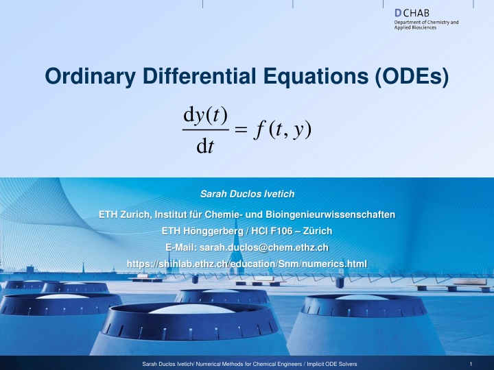
Ordinary Differential Equations (ODEs) d ( ) d y t = ( , ) f t y t Sarah Duclos Ivetich ETH Zurich, Institut f r Chemie- und Bioingenieurwissenschaften ETH H nggerberg / HCI F106 Z rich E-Mail: sarah.duclos@chem.ethz.ch https://shihlab.ethz.ch/education/Snm/numerics.html Sarah Duclos Ivetich/ Numerical Methods for Chemical Engineers / Implicit ODE Solvers 1
Runge-Kutta methods If we approximate the slope field more accurately between two iteration steps, we can generate methods higher local and global accuracy orders Approximating the slope field in m stages: ( ) ( ) ( ( 3 3 31 1 32 2 , n n k f t hc y h a k a k = + + + = = , k f t y 1 n n hc y + + , k f t ha k Nodes Weights Runge-Kutta Matrix c b a 2 2 21 1 n n i ) ) i ij 1 m Slopes Number of stages k m = + + , k f t hc y h mi i a k i m n m n = 1 i m = + y y h b k + 1 n n j j = 1 j Sarah Duclos Ivetich / Numerical Methods for Chemical Engineers / Implicit ODE Solvers 2
Butcher tableau A convenient way of of writing down explicit RK methods is the Butcher tableau Example: Heun, order 2 0 c c 0 1 a a 2 21 1 a 3 31 32 1 2 1 2 c a b a b a b ( ( y ) , = = , k f t y 1 2 1 m m m mm 1 n n h y b ) + + 1 2 1 m m k f t = hk + 2 1 1 2 n n ( ) + 1 2 y h k k + 1 1 2 n n Sarah Duclos Ivetich / Numerical Methods for Chemical Engineers / Implicit ODE Solvers 3
0 c c a a 2 21 a Visualization of RK methods 3 31 32 c a b a b a b 1 2 1 m m m mm b 1 2 1 m m Nodes Weights Runge-Kutta Matrix c b a ( ( ) = = i , k f t y m 1 n n hc y = + i y y h b k ) + + + 1 n n j j , k f t ha k ij = 2 2 21 1 n n 1 j Slopes Number of stages k m i ny+ 1 2k + y ha k 21 1 1k ny nt nt+ + nt hc 1 2 Sarah Duclos Ivetich / Numerical Methods for Chemical Engineers / Implicit ODE Solvers 4
Interpolation of end value t0 t1 t2 t3 tn-3 tn-2 tn-1 tn tend tn+1 Sarah Duclos Ivetich / Numerical Methods for Chemical Engineers / Implicit ODE Solvers 5
Assigment 1: Radioactive decay A decaying radioactive element changes its concentration according to the ODE d ( , ) d t y = = f t y y where is the decay constant The analytical solution to this problem reads ( ) ( ) = y t y t 0exp Sarah Duclos Ivetich / Numerical Methods for Chemical Engineers / Implicit ODE Solvers 6
Assignment 1: Radioactive decay You have implemented the forward Euler method The forward Euler method reads The backward Euler algorithm uses the following step formula 1 n n y y h f t ( ) += h f t y + , y y 1 n n n n ( ) = + , y + + + 1 1 n n Note that you cannot just put this formula into Matlab like this! Use fsolve to solve for with the same conditions as above. You might want to use these to avoid spamming you command line: options = optimset('display','off'); y(i+1) = fsolve( ........, options); Sarah Duclos Ivetich / Numerical Methods for Chemical Engineers / Implicit ODE Solvers 7
Assigment 1: Radioactive decay 0 1 2 1 2 0 Butcher tableaus can be read as: Heun2: 1 1 RK4: 1 2 0 0 1 6 1 3 1 3 1 6 1 2 0 ( ( ( ) = = = , k k k f t y f t f t 1 2 1 2 1 1 1 n n hc y hc y ) + + + + , , ha k h a k 0 c c 2 2 21 1 n n ) ( ) + 32 2 a k a a 3 3 31 1 n n 2 21 a 0 1 2 1 2 3 31 32 1 1 2 1 2 1 m 0 = + + , k f t hc y h Heun2: 1 mi i a k m n m n c a b a b a b RK4: 1 2 0 0 1 6 1 3 1 3 1 6 1 2 0 = 1 i 1 2 1 m m m mm b 1 1 m 1 2 1 m m = + y y h b k + 1 n n j j = 1 j Solve the radioactive decay problem using the 2nd order Heun method and the 4th order RK method using the conditions y0 = 1, lambda = 1 and h = 0.1 from t0 = 0 to tEnd = 10 Define 4 new functions such function [t,y] = eulerForward(f,t0,tend,y0,h) function [t,y] = eulerBackward(f,t0,tend,y0,h) function [t,y] = Heun2(f,t0,tend,y0,h) function [t,y] = RK4(f,t0,tend,y0,h) to be called in your main code Sarah Duclos Ivetich / Numerical Methods for Chemical Engineers / Implicit ODE Solvers 8
Assigment 1: Radioactive decay Note that you cannot just put the backward Euler formula into Matlab! Use fsolve to solve for ??+1 with the same conditions as for the forward Euler. You might want to use these to avoid spamming you command line: options = optimset('display','off'); y(i+1) = fsolve( ........, options); As shown in slide 5, discretize your integration steps until tEnd+h and interpolate the final value between tEnd and tEnd+h. Compare the orders of accuracy for the four methods (Forward and Backward Euler, 2nd order Heun and 4th order RK) plotting the global truncation errors of the last element defined as ??= ? ?? ?? against h with h = logspace(-4,0,8) in a double logarithmic plot (loglog). Note that a method has order of accuracy p if ??= ? ?. Sarah Duclos Ivetich / Numerical Methods for Chemical Engineers / Implicit ODE Solvers 9
Assignment 2 The van der Waals equation for some non-ideal gas reads 2.4 3 = P ( ) 2 1 3 V V Taking the derivative, we get d d 6 2.4 1 3 P V = ( ) 2 3 V V Sarah Duclos Ivetich / Numerical Methods for Chemical Engineers / Implicit ODE Solvers 10
Assignment 2 (continued) 1. Plot the van der Waals equation for 1000 points between V = 0.34 and V = 4 2. Try to approximate the equation by solving the ODE Use ode45, tSpan = [0.34, 4]; and y0 = P(0.34); Note that the ODE does not depend on the solution, but only the independent variable (i.e. the first input into your odefun!) Plot the solution of the ODE together with the analytical solution and zoom in to ylim([0, 2]). What do you observe? Try the same with ode15. What do you observe when you zoom in? 3. Plot dP/dV against V in the range we considered. What might be the problem with the solvers, considering what they have to do in the slope field? 4. Tighten the tolerances. Plot the solutions again and zoom in to ylim([0,2]). Sarah Duclos Ivetich / Numerical Methods for Chemical Engineers / Implicit ODE Solvers 11
Assignment 3 Compute the stability function of the Runge method (also known as the explicit midpoint method (EM)). Sarah Duclos Ivetich / Numerical Methods for Chemical Engineers / Implicit ODE Solvers 12
