Industrial Engineering Lecture IV: Design of Experiments and Probability Distributions
Explore the world of Industrial Engineering through Lecture IV by Dr. Adham Ragab, delving into the basics of normal distribution, random variables, probability mass functions, and more. Gain insights into the differences between discrete and continuous probability distributions, understanding the normal distribution, and utilizing normal distribution tables.

Download Presentation

Please find below an Image/Link to download the presentation.
The content on the website is provided AS IS for your information and personal use only. It may not be sold, licensed, or shared on other websites without obtaining consent from the author. If you encounter any issues during the download, it is possible that the publisher has removed the file from their server.
You are allowed to download the files provided on this website for personal or commercial use, subject to the condition that they are used lawfully. All files are the property of their respective owners.
The content on the website is provided AS IS for your information and personal use only. It may not be sold, licensed, or shared on other websites without obtaining consent from the author.
E N D
Presentation Transcript
Industrial Engineering Design of Experiments (Lecture IV) Dr. Adham Ragab
Industrial Engineering Outline Review of normal distribution basics.
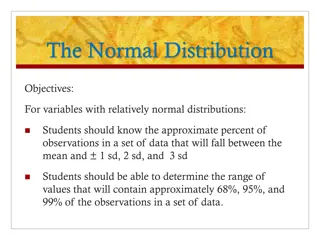
Industrial Engineering Objectives By the end of this lecture the student should be able to: Recognize the differences between discrete and continuous probability distribution. Understand the normal distribution Use normal distribution tables
Random Variables Industrial Engineering Random Variable (RV): A numeric outcome that results from an experiment The description of the possible values of a random value X and the probabilities of each has a name: the probability distribution.
Industrial Engineering PMF Discrete random variable is one whose possible values form a discrete set The probability distribution of a discrete random variable is called: Probability Mass Function
Example I Rolling 2 Dice (Red/Green) Industrial Engineering Y = Sum of the up faces of the two die. Table gives value of y for all elements in S Red\Gree n 1 1 2 3 4 5 6 2 3 4 5 6 7 3 4 5 6 7 8 4 5 6 7 8 9 5 6 7 8 9 10 6 7 8 9 10 11 7 8 9 10 11 12 2 3 4 5 6
Industrial Engineering Rolling 2 Dice Probability Mass Function & CDF y 2 3 4 5 6 7 8 9 p(y) 1/36 2/36 3/36 4/36 5/36 6/36 5/36 4/36 3/36 2/36 1/36 F(y) 1/36 3/36 6/36 10/36 15/36 21/36 26/36 30/36 33/36 35/36 36/36 # of ways 2 die can sum to y = ( ) p y # of ways 2 die can result in y = t = F(y) p(t) 2 CDF= Cumulative Distribution Function 10 11 12
Rolling 2 Dice Probability Mass Function Industrial Engineering Dice Rolling Probability Function 0.18 0.16 0.14 0.12 0.1 p(y) 0.08 0.06 0.04 0.02 0 2 3 4 5 6 7 8 9 10 11 12 y
Rolling 2 Dice Cumulative Distribution Function Industrial Engineering Dice Rolling - CDF 1 0.9 0.8 0.7 0.6 F(y) 0.5 0.4 0.3 0.2 0.1 0 1 2 3 4 5 6 7 8 9 10 11 12 13 y
Industrial Engineering Example II A company produces aluminum sheets. The sheet is considered defected if the number of flaws exceeds 2. The probability mass function is shown in the figure. What is the expected defect rate of the produced sheets?
Industrial Engineering Probability Mass Function
Industrial Engineering PDF A continuous random variable is one whose possible values form a continuous set. The probability distribution of a continuous random variable is called: Probability density Function
Industrial Engineering PDF, cont. Probability determined from the area under f(x).
Industrial Engineering PDF, cont. Definition http://civil.colorado.edu/~balajir/CVEN5454/lectures/ch04.ppt
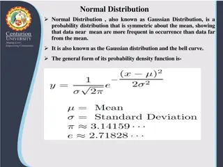
Industrial Engineering The Normal Distribution The normal distribution (also called the Gaussian distribution) is by far the most commonly used distribution in statistics. This distribution provides a good model for many, although not all, continuous populations. The normal distribution is continuous rather than discrete. The mean of a normal population may have any value, and the variance may have any positive value. 15
Normal R.V.: pdf, mean, and variance The probability density function of a normal population with mean and variance 2 is given by 1 ( ) , 2 Industrial Engineering = 2 2 ) /2 ( f x e x x https://www.youtube.com/watch?v=VQepRP-f6GA 16
68-95-99.7% Rule Industrial Engineering This figure represents a plot of the normal probability density function with mean and standard deviation . Note that the curve is symmetric about , so that is the median as well as the mean. It is also the case for the normal population. About 68% of the population is in the interval . About 95% of the population is in the interval 2 . About 99.7% of the population is in the interval 3 . 17
Industrial Engineering Standard Normal Distribution In general, we convert to standard units by subtracting the mean and dividing by the standard deviation. Thus, if x is an item sampled from a normal population with mean and variance 2, the standard unit equivalent of x is the number z, where z = (x - )/ . The number z is sometimes called the z-score of x. The z-score is an item sampled from a normal population with mean 0 and standard deviation of 1. This normal distribution is called the standard normal distribution. 18
Industrial Engineering Normal Distribution Normal probability density functions for selected values of the parameters and 2. http://civil.colorado.edu/~balajir/CVEN5454/lectures/ch04.ppt
Industrial Engineering Example Aluminum sheets used to make beverage cans have thicknesses that are normally distributed with mean 10 and standard deviation 1.3 thousandths of inches. A particular sheet is 10.8 thousandths of an inch thick. Find the z-score. 20
Industrial Engineering Example The thickness of a certain sheet has a z- score of -1.7. Find the thickness of the sheet in the original units of thousandths of inches. 21
Industrial Engineering Examples Find the area under normal curve to the left of z = 0.47. 22
Industrial Engineering Examples Find the area under the curve to the right of z = 1.38.
Industrial Engineering Example 4.43 Find the area under the normal curve between z = 0.71 and z = 1.28. 24
Industrial Engineering Summary Normal distribution is the most common probability distribution used in statistics. Any normal distribution could be transformed to a standard normal distribution for the convenience of using the tables.


")