Inference of Urban Water Storage Capacity from Evapotranspiration Recession Analysis
A new method is proposed to estimate urban water storage capacity based on evapotranspiration recession analysis, showcasing the significant differences between urban and rural/forested areas. The study highlights the strong water limitations in cities, leading to smaller water storage capacities. Figures and tables illustrate the application of recession analysis to evapotranspiration observations in various cities, providing insights into water storage dynamics. The research emphasizes the importance of understanding urban water systems for sustainable urban planning and water resource management.

Download Presentation

Please find below an Image/Link to download the presentation.
The content on the website is provided AS IS for your information and personal use only. It may not be sold, licensed, or shared on other websites without obtaining consent from the author.If you encounter any issues during the download, it is possible that the publisher has removed the file from their server.
You are allowed to download the files provided on this website for personal or commercial use, subject to the condition that they are used lawfully. All files are the property of their respective owners.
The content on the website is provided AS IS for your information and personal use only. It may not be sold, licensed, or shared on other websites without obtaining consent from the author.
E N D
Presentation Transcript
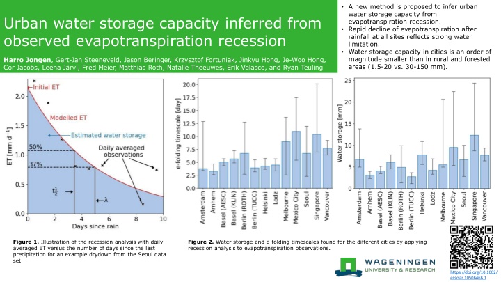
A new method is proposed to infer urban water storage capacity from evapotranspiration recession. Rapid decline of evapotranspiration after rainfall at all sites reflects strong water limitation. Water storage capacity in cities is an order of magnitude smaller than in rural and forested areas (1.5-20 vs. 30-150 mm). Urban water storage capacity inferred from observed evapotranspiration recession Harro Jongen, Gert-Jan Steeneveld, Jason Beringer, Krzysztof Fortuniak, Jinkyu Hong, Je-Woo Hong, Cor Jacobs, Leena J rvi, Fred Meier, Matthias Roth, Natalie Theeuwes, Erik Velasco, and Ryan Teuling Figure 1. Illustration of the recession analysis with daily averaged ET versus the number of days since the last precipitation for an example drydown from the Seoul data set. Figure 2. Water storage and e-folding timescales found for the different cities by applying recession analysis to evapotranspiration observations. https://doi.org/10.1002/ essoar.10506466.1
Figure 3. Daily average ET versus the day after the last precipitation with in red (continuous) the recession curve using the median parameter values, in blue (dotted) the 5thand 95thpercentile of the median distribution from the bootstrapping re-samples, and in light grey all individual drydowns. The parameters of the fitted curves are shown in Table 1.
Table 1. Summary of the measurement sites and the outcomes of the regression. (LCZ: 1 = compact high-rise, 2 = compact mid-rise, 3 = compact low-rise, 5 = open mid-rise, 6 = open low-rise, Fv: surface fraction covered by vegetation in a 500 m radius around the measurement site, zs: height of sensors above ground level, zH: mean building height, ET0: initial evapotranspiration, : e-folding timescale, t1 2: half-life, S0: water storage capacity K ppen- Geiger climate Fv (%) zs (m) zH (m) ET0 (mm d-1) (day) S0 (mm) t1 2 City LCZ Dry-downs Days Amsterdam Cfb 2 15 40 14 14 56 0.99-2 (1.5) 3.4-7.3 (3.8) 2.4-10 (2.6) 5.6-17 (6.7) Arnhem Cfb 2 12 23 11 48 195 0.62-0.95 (0.73) 2.6-4.6 (3.3) 1.8-3.2 (2.3) 2.4-3.9 (3.1) Basel (AESC) Cfb 2 27 39 17 125 523 0.76-1 (0.83) 4.4-5.7 (5) 3.1-3.9 (3.5) 3.5-4.8 (4) Basel (KLIN) Cfb 2 27 41 17 160 685 0.9-1.2 (1) 5-7 (5.7) 3.5-4.9 (3.9) 4.7-7.7 (6.1) Berlin (ROTH) Cfb 6 56 40 17 8 36 0.46-0.95 (0.74) 4.1-12 (6.7) 2.8-8.1 (4.7) 2-9.7 (4.9) Berlin (TUCC) Cfb 5 31 56 20 38 153 0.31-0.78 (0.47) 3.3-5.1 (3.9) 2.3-3.5 (2.7) 1.2-3.6 (2.7) Helsinki Dfb 6 54 31 20 45 197 1.1-1.8 (1.6) 3.7-5.3 (4.3) 2.5-4 (3) 5.6-11 (7.8) d Dfb 5 31 37 11 59 269 0.74-1.4 (1) 3.6-5.3 (4.5) 2.5-3.8 (3.1) 3.4-6.7 (4.2) Melbourne (Preston) Cfb 5 38 40 6 3 12 0.55-2.1 (1.5) 2.6-14 (9) 1.8-9.5 (6.2) 5-21 (5.5) Mexico City Cwb 2 6 37 9.7 8 49 0.69-1.5 (1.2) 5.4-17 (11) 3.8-11 (7.6) 5.8-22 (9.5) Seoul Dwa 1 40 30 20 11 66 0.74-1.7 (1.1) 2.8-11 (6.7) 2-7.3 (4.7) 3.1-9.9 (6.7) Singapore Af 3 15 24 10 7 41 1.2-1.6 (1.3) 7-20 (10) 4.8-14 (7.2) 8.7-24 (12) Vancouver Csb 6 35 28 5 63 293 1-1.4 (1.2) 6.8-9.1 (7.7) 4.7-6.3 (5.4) 6.6-8.9 (7.7)
Figure 4. The seasonal cycle of S0for the sites on the northern hemisphere (Melbourne is included shifted by half a year) in blue and for Singapore as grey dots. The uncertainty is determined similarly as in Figure 3.