Innovative 60 GHz Channel Model for D2D Links in IEEE 802.11

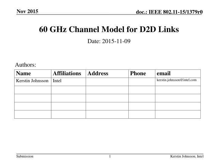
Nov 2015 doc.: IEEE 802.11-15/1379r0 60 GHz Channel Model for D2D Links Date: 2015-11-09 Authors: Name Kerstin Johnsson Intel Affiliations Address Phone email kerstin.johnsson@intel.com Submission 1 Kerstin Johnsson, Intel

Nov 2015 doc.: IEEE 802.11-15/1379r0 Abstract This presentation introduces a stochastic 60 GHz channel model for D2D links. Submission 2 Kerstin Johnsson, Intel

Nov 2015 doc.: IEEE 802.11-15/1379r0 Outline Introduction - Applicable usage models - Channel modeling goals - Limitations of existing models Overview of proposed channel model - Concept, advantages, limitations Channel model implementation - Key operations - Performance Conclusions Submission 3 Kerstin Johnsson, Intel

Nov 2015 doc.: IEEE 802.11-15/1379r0 Applicable 802.11ay Usage Models Channel model was originally designed for AR/VR Headsets, High-End Wearables Also applies to other D2D-based models: 8K UHD Wireless Transfer Office Docking https://encrypted-tbn1.gstatic.com/images?q=tbn:ANd9GcRLC5R5iSEz6MmQwFi4lrD0g7MG_1WyLuPFTSIbqQl1VFj1ajfDe4I0-g Wireless transfer from fixed device Set-top box (TV controller) https://encrypted-tbn3.gstatic.com/images?q=tbn:ANd9GcTIjdwqNoeakwq05XWf0cSoY9zD3wh9G-ykSTDk-CGB0PXQ11IYsK2a4QM http://c.dryicons.com/images/icon_sets/travel_and_tourism_part_2/png/512x512/wifi.png Blu-ray player http://c.dryicons.com/images/icon_sets/travel_and_tourism_part_2/png/512x512/wifi.png http://c.dryicons.com/images/icon_sets/travel_and_tourism_part_2/png/512x512/wifi.png https://encrypted-tbn3.gstatic.com/images?q=tbn:ANd9GcQhHQMNWdGnqAK1ekRNjfgs8cg9uRghIdJRIJ0qMAgUMrcjNQ3o3YPbDJo Smartphone/ Tablet Submission 4 Kerstin Johnsson, Intel

Nov 2015 doc.: IEEE 802.11-15/1379r0 Goals for the new channel model Capabilities Provide complete CSI, e.g. complex impulse response, AoA, AoD, etc. Accurate for arbitrary link distances > 30cm Maintain spatial and temporal correlations Model self-blocking (hands, arms, etc.) Results are reproducible (based on the same seed) Speed Thousands of samples per second Simplified environment representation (no 3D CAD models) Submission 5 Kerstin Johnsson, Intel

Nov 2015 doc.: IEEE 802.11-15/1379r0 Limitations of conventional models Most conventional channel models (HATA, ITU etc) are simple: The trend is fitted to a log-distance model Fluctuations around the trend are represented as random processes Typically, two processes are used: Distance-dependent, frequency-flat (slow fading) Time-dependent, frequency-correlated (fast fading) For mmWave, this channel information is not sufficient Submission 6 Kerstin Johnsson, Intel

Nov 2015 doc.: IEEE 802.11-15/1379r0 Grid-based extensions (3GPP/IEEE) Environment partitioned into a grid and assigned shadow fading values using log- normal distribution parametrized for environment For a given location, shadow fading is calculated by interpolating between grid values, thereby maintaining spatial correlation (note: value is same regardless of antenna orientation, TX/RX heights, etc.) Fast fading is added based on standard Rayleigh/Rician distribution, i.e. not directly connected to user movement Grid box size is proportional to de-correlation distance Cellular frequencies require ~ 10m gridbox mmWave frequencies require ~ 0.1m gridbox (huge amount of data!) Submission 7 Kerstin Johnsson, Intel

Nov 2015 doc.: IEEE 802.11-15/1379r0 Using Ray Tracing to populate 3D grid Standard large/small scale fading models do not fully capture mmWave channel - only ray tracing can provide necessary detail An accurate 3D environment grid for mmWave requires: One full 3D environment grid for each potential TX location! Gridbox dimensions < 10x10x10 cm To determine received signal in every gridbox of a 5x5x2.5m room for one given TX location requires 62500 ray tracing runs! We need a faster, more efficient method - can we reproduce results stochastically? Submission

Nov 2015 doc.: IEEE 802.11-15/1379r0 Outline Introduction - Applicable usage models - Channel modeling goals - Limitations of existing models Overview of proposed channel model - Concept, advantages, limitations Channel model implementation - Key operations - Performance Conclusions Submission 9 Kerstin Johnsson, Intel

Nov 2015 doc.: IEEE 802.11-15/1379r0 Channel Model At the receiver, the channel is a superposition of multipath components [MPC] MPC can be characterized by: full 3D trajectory (including all reflections/diffractions) reflection/absorption/interaction loss initial power is equal to the TX power Our channel model reproduces MPCs stochastically Preserves statistics of the sample environment Equivalent to ray tracing in level of detail With MPC information, we can calculate: Path loss MIMO capacity Impulse response subject to given antenna Submission Slide 10 Kerstin Johnsson, Intel * MPC models assume isotropic TX and RX

Nov 2015 doc.: IEEE 802.11-15/1379r0 Modeling MPCs For any given TX/RX pair, ray tracing tells us: How many MPCs constitute the channel? (3 in the example) How many interactions happened per MPC (i.e. what is its order)? Where did the interactions happen? (points C, D, E, F in the example) What were the associated interaction losses? MPCs are unique for each TX/RX pair, but MPCs should be spatially and temporally correlated. MPC data is collected for sample environment; statistics are then drawn from the data and used to generate MPCs stochastically Submission 11 Kerstin Johnsson, Intel

Nov 2015 doc.: IEEE 802.11-15/1379r0 Processing of channel model output MPC power is adjusted based on TX/RX antenna gains (models beamforming) Impulse response [IR] is generated (weak components may be ignored) IR is sampled at carrier frequency (capturing interference between MPCs) ISI can be directly measured (based on symbol duration) FFT of IR yields full CSI for OFDM Coupling loss can be computed (for automatic gain control, power control tests) But how do we produce the MPCs? Submission 12 Kerstin Johnsson, Intel

Nov 2015 doc.: IEEE 802.11-15/1379r0 Limitations of the model The geometry of the environment can not be too simple Randomness in the environment is good! The environment should be statistically isotropic Density of objects should not vary significantly One could extend the model to lift those restrictions Submission 13 Kerstin Johnsson, Intel

Nov 2015 doc.: IEEE 802.11-15/1379r0 Outline Introduction - Applicable usage models - Channel modeling goals - Limitations of existing models Overview of proposed channel model - Concept, advantages, limitations Channel model implementation - Key operations - Performance Conclusions Submission 14 Kerstin Johnsson, Intel

Nov 2015 doc.: IEEE 802.11-15/1379r0 Channel model implementation 1. Use ray tracing to evaluate channel for large enough number of TX/RX locations to fully capture sample environment 2. For a given TX/RX pair, stochastically reproduce MPCs as follows: Calculate number of MPCs of each order (LOS, 1st, 2nd, etc.) based on TX- RX distanceand identify each MPC s interaction points (yields trajectory) Reproduce each MPC s losses Compute the power and delay of each MPC Apply smoothing to model diffraction 3. Apply necessary corrections (e.g. body blockage loss for wearables) 4. Reconstruct impulse response, run post-processing Compute effective RSS, ISI, frequency response, etc. Submission 15 Kerstin Johnsson, Intel

Nov 2015 doc.: IEEE 802.11-15/1379r0 Processing ray tracing data Learning data comes from statistically large number of random TX/RX links Based on learning data we can compute: How many MPCs of each order are present for various TX/RX link lengths Distribution of hop lengths and mutual angles for various TX/RX link lengths Angle-dependent interaction loss statistics Correlation distances in various directions Other statistics as necessary Submission 16 Kerstin Johnsson, Intel

Nov 2015 doc.: IEEE 802.11-15/1379r0 Reproducing MPCs the challenge Each MPC is shaped by one or more interaction sources E.g. reflective wall May come in and out of view Will appear at different angles depending on point of view With TX/RX movement, interaction sources appear and disappear We approximate visibility of interaction sources w/ Boolean function (similar function used to determine visibility of LOS component) Any number of interaction sources may be active in the channel With ray tracing all interactions are coupled to geometry (complex) With stochastic model interactions are drawn randomly and independently Average number of active interaction points depends on TX-RX distance Interaction sources stay active within a certain area to ensure proper correlation Submission 17 Kerstin Johnsson, Intel

Nov 2015 doc.: IEEE 802.11-15/1379r0 Reproducing MPCs the model Interaction sources are only visible to RX when in certain areas of environment Areas change as TX moves (requiring significant processing and data storage!) We model interaction sources and their visibility using statistics from ray tracing Create stationary interaction points (not 1:1 mapped with original interaction sources) and mobile activations areas that move w/ TX and RX Overlap of activation area and interaction point represents an interaction for the MPC Size of an activation area encodes correlation distance Submission 18 Kerstin Johnsson, Intel

Nov 2015 doc.: IEEE 802.11-15/1379r0 Reproducing MPCs the statistics Ray tracing tells us the mean and variance of the number of MPCs of each order present for a TX-RX link of a given distance Average and variance of the number of nth order MPCs is modeled by varying the: density of activation areas in the environment (p) number of interaction points in the environment (N) LOS is simply modeled as existing (or not) based on ray tracing statistics Submission 19 Kerstin Johnsson, Intel

Nov 2015 doc.: IEEE 802.11-15/1379r0 Reproducing MPCs an example Assume RX is moving toward TX Two 1st order MPCs are possible As RX moves, activation areas move overlapping the two possible interaction points at different times (each overlap represents the activation of a 1st order MPC) Submission 20 Kerstin Johnsson, Intel

Nov 2015 doc.: IEEE 802.11-15/1379r0 Reproducing MPCs - summary Now we can generate Presence of LOS path between the given TX/RX pair Interaction points for the NLOS paths present between the TX/RX pair This data will have the Correct spatial correlations for the generated MPCs as TX and/or RX moves Correct variances and means of 1st, 2nd, 3rd, etc. order MPCs Correct cross-correlations between mean/variance in number of 1st, 2nd, 3rd, etc. order MPCs Using this data, we now generate each MPC s trajectory and interaction losses Submission 21 Kerstin Johnsson, Intel

Nov 2015 doc.: IEEE 802.11-15/1379r0 Producing MPC trajectories For each possible MPC order (LOS, 1st, 2nd, etc.), create a matrix from the ray tracing data of all MPCs of the given order where: Each column is an nth order MPC from the ray tracing data Rows represent the 3D vectors between the Rx and Tx followed by the hop vectors to each interaction point, thus for a 2nd order MPC the column vector would be [xRx - xTx, yRx - yTx, zRx - zTx, x1 - xTx, y1 - yTx, z1 - zTx, x2 - x1,y2 - y1, z2 - z1] ) Compute covariance matrix ? For a normally distributed random vector ?, covariane of ? = ? ? is same as ? Problem is, ? represents random Tx and Rx locations To create a ? vector that represents a Tx/Rx pair with a specific = ?? ?? Pre-generate ? 1:3,1 = ? ?, ? [4:???,1] = ?????(), where seed is set to the no. of interaction points Now ? = (? ? ) will have the of our choosing! Submission 22 Kerstin Johnsson, Intel

Nov 2015 doc.: IEEE 802.11-15/1379r0 Producing MPC trajectories results All trajectories are statistically equivalent to ray tracing data in every aspect Multiple vectors based on the same Tx/Rx can be considered for MIMO Submission 23 Kerstin Johnsson, Intel

Nov 2015 doc.: IEEE 802.11-15/1379r0 Special case: self-blocking Normally, in a highly random environment, LOS is guaranteed as Tx/Rx distance goes to 0 In practice, this is not the case; often the user is the major blocker Human bodies cause significant attenuation (> 60dB from palm alone) LOS path may be significantly attenuated by antenna polarization mismatch as well Need to override LOS probability at very short ranges (< 50 cm) This should be done on case-by-case basis If the blockage does happen, we can still apply the NLOS model Submission 24 Kerstin Johnsson, Intel

Nov 2015 doc.: IEEE 802.11-15/1379r0 Special case: partial body blocking Difficult to occlude entire mmWave beam with e.g. an arm Depends on the antenna s aperture, position of arm relative to TX/RX antennas, etc. Partially-blocked links can be considered LOS Simple model can be used to capture extra attenuation Submission 25 Kerstin Johnsson, Intel

Nov 2015 doc.: IEEE 802.11-15/1379r0 Putting it all together Calculate no. of 1st, 2nd, 3rd, etc. order MPCs for given TX/RX pair based on link distance Determine trajectory of each MPC Calculate power of each MPC = TX power - free space loss - interaction losses + antenna gains Convolve MPCs with a sampled sinc function System bandwidth affects the period of the sinc function Doppler may be added based on TX and RX speeds All sincs are then multiplied by their complex phase Phase encodes the time of arrival Submission 26 Kerstin Johnsson, Intel

Nov 2015 doc.: IEEE 802.11-15/1379r0 NLOS fading comparisons Simulated multipath shows patterns similar to real one! Submission 27 Kerstin Johnsson, Intel

Nov 2015 doc.: IEEE 802.11-15/1379r0 SNR comparisons Based on 60 GHz channel measurement campaign: For each TX/RX channel measurement, the values from the best antenna orientations were recorded Data for both NLOS and LOS was collected Measured 50 cm phone-to-head links with varying head/body positions Assumed 62dB free space loss Scenario type Measured, dB (Min/Max) Model, dB (Min/Max) Rich multipath, LOS -60/-64 -57/-69 Rich multipath, NLOS -67/-85 -65/-83 Poor multipath, LOS -62/-67 -62/-64 Poor multipath, NLOS 85 / 90 86 / -- (90% quantiles are given for min & max values) Submission 28 Kerstin Johnsson, Intel

Nov 2015 doc.: IEEE 802.11-15/1379r0 Outline Introduction - Applicable usage models - Channel modeling goals - Limitations of existing models Overview of proposed channel model - Concept, advantages, limitations Channel model implementation - Key operations - Performance Conclusions Submission 29 Kerstin Johnsson, Intel

Nov 2015 doc.: IEEE 802.11-15/1379r0 Conclusions The proposed model effectively replaces ray tracing Full 3D impulse response is generated MIMO & beamforming data can be easily extracted Accurate spatial correlations are maintained Deterministic operation Coherence distance explicitly modeled Low computational complexity Most operations are basic vector algebra Ray tracing based data has been compressed and can be provided High flexibility Arbitrary scenarios can be represented Other frequencies can be supported Submission 30 Kerstin Johnsson, Intel