Innovative Network Structures and Solitary Waves on Tensegrity Prisms
Spatial reticulate systems in self-stress, tensegrity configurations with rigid bodies, and dynamic responses to impulsive loads are explored in this workshop on innovative network structures interacting with solitary waves, conducted at the University of Salerno.

Download Presentation

Please find below an Image/Link to download the presentation.
The content on the website is provided AS IS for your information and personal use only. It may not be sold, licensed, or shared on other websites without obtaining consent from the author.If you encounter any issues during the download, it is possible that the publisher has removed the file from their server.
You are allowed to download the files provided on this website for personal or commercial use, subject to the condition that they are used lawfully. All files are the property of their respective owners.
The content on the website is provided AS IS for your information and personal use only. It may not be sold, licensed, or shared on other websites without obtaining consent from the author.
E N D
Presentation Transcript
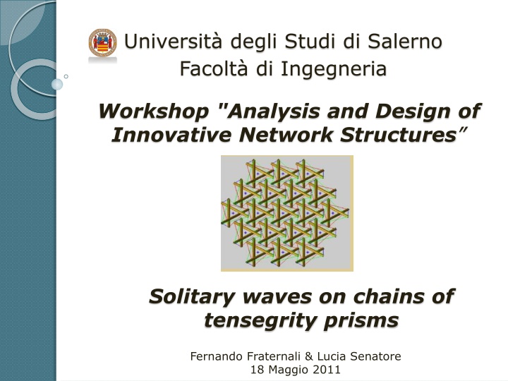
Universit degli Studi di Salerno Facolt di Ingegneria Workshop "Analysis and Design of Innovative Network Structures Solitary waves on chains of tensegrity prisms Fernando Fraternali & Lucia Senatore 18 Maggio 2011
OVERVIEW 1) Introduction 2) Constitutive behavior a 3-bar tensegrity prism 3) Basic notions on solitary waves 4) Wave analysis 5) Strength Analysis 6) Concluding remarks
Part 1: INTRODUCTION TENSEGRITY is a spatial reticulate system in a state of self-stress. The structure is based on the combination of a few patterns: Loading members only in pure compression or pure tension, meaning the structure will only fail if the cables yield or the rods buckle. Preload or tensional prestress, which allows cables to be rigid in tension. Mechanical stability, which allows the members to remain in tension/compression as stress on the structure increases
A tensegrity configuration can be established when a set of tensile members are connected between rigid bodies. Classes of tensegrity systems Class I A single rigid element in each node One tensile element connecting the two rigid bodies Class II Rigid body Two rigid elements in each node Two tensile elements connecting the two rigid bodies
Rigid body Class III Three rigid elements in each node Three tensile elements connecting the three rigid bodies Class III Class I Class II
Regular minimal tensegrity prism Tensegrity structure with minimum number of strings equal to 9 Regular non-minimal tensegrity prism Tensegrity structure with number of strings major than the minimum
Research goals It has been shown that 1-D systems featuring non linear force-displacement response, like, e.g, systems with power law, tensionless response (Nesterenko, 2001, Daraio et al., 2006), support energy transport through solitary waves. We prove with this study that a similar behavior is exhibited by 1-D chains of class-1 tensegrity prisms in unilateral contact each other, through a numerical approach. We study the dynamic response of such systems to impulsive loads induced by the impact with external strikers , through numerical integration of the equations of motions of the individual prisms
An initial analytic study leads us to model each prism as a non linear 1-D spring , which exhibits a locking type response under sufficiently large compressive forces. The analysis of the steady state wave propagation regime allows us to detect the localized nature of the traveling waves, and the correlations occurring between the wave speed, the maximum transmitted force, the maximum axial strain, and the wave width. By examining different material systems, we find that the locking regime supports solitary waves with atomic-scale localization of the transported energy. We conclude the present study with a discussion of the given results, and the analysis of the possible future extensions of the current research.
Part 2 : Constitutive behavior of a 3-bar tensegrity prism
2.1 Schematic of a 3-bar tensegrity prism Characteristic transverse dimension a L Cross-cable length Bar length Twist angle between upper and lower bases h p Prism height Axial strain a a h Natural length of cross-cables N Cable prestrain ck m Cable stiffness Total prism mass Elastic stiffness of the prism at equilibrium (zero axialforce) 0 k m Fundamental vibration period of the prism = 2 T 0 k 0
2.2 Kinematics B Lower basis a Legs: A- B- C- b c c a 3 a 2 c a b Cross-cables : A- B- C- 150 A 3 a 2 Upper basis C b a a 2
B Lower base c a Legs: A- B- B- C- C- c Cross-cables : A- a b b a c 3 a 2 150 Position vectors (upper base) e h P 3 , , = A + Q P 3 , , a b c A B C a 2 cos sin 0 Upper base = Q C sin cos 0 b a 0 0 1 a 2 Fixed length constraint on the legs = 2 2 ( ) P P L , , , , a b c A B C a 2 2 L h = = 2 2 2 1 ( cos ) arccos 1 h L a (1) 2 2 Cross- cable length (2) = = + 2 2 2 ( ) 3 ( cos 3 sin ) P P L a , , a b c , , B C A
2.3 Force-displacement relationship 2.3.1 Direct approach Fa Nac-- - Fc c - a Equilibrium equations NaA - = + + + + = ) 0 a F N N N N a a A a c a B a b NaB - Ncb-- Nab-- NcC- = + + + + = ) 0 b F N N N N Fb b b B a b C b c b - NcA- b NbB - = + + + + = ) 0 c F N N N N c c C a c c A c b B NCb- A C
Assuming vertical loading Fa= {0 , 0 , -Fa} , Fb= {0 , 0 , -Fb} , Fc= {0 , 0 , -Fc} and elastic behavior of the cross-cables = = = ( ) N N N k a C c B N b A , , , , , F F F N N N we can solve (9 scalar equations) for ), ), c b a ) a b c a A c C b B , , N N N a c a b b c = (h ) In particular, by setting we obtain the overall force vs height relationship as : = + + ( ) ( ( ) ( ) ( )) F h F h F h F h a b c
2.3.2 Energetic approach Elastic energy 3 = 2) ( ) ( U k N 2 By using (1) and (2) we can express U as a function of or h Torque ( d ( ) ) dU = = ( 3 ) M k d d N Axial force (assuming as positive compressive forces) ( ) ( ) dU h d h = = 3 ( ) F k N dh dh
2.4 Equilibrium values of the twist angle, prism height and cable length ( ) dU solution of 0 = = 0 M (3) d ( ) dU h 0 h = = solution of 0 F (4) dh By solving (3), we get 5 = (150 ) 0 6 = 2 1 ( cos ) 2 2 h L - a 0 0 = 2 3 2 2 L - a 0
2.5 Force vs height relationship Upon writing + = = 0 0 N p N p 1 N where p is the cable prestrain, we get for U(h) and F(h) the following expressions : 2 + 2 2 2 3h 6 ( 3 ( )) L a c h 3 = 0 ( ) k 2 U h + 1 p 2 + + 3 6 ( 3 ( ) 2 2 2 h L a c h 2 ( 3 ) 2 2 2 a h L + 3 3 hk 0 + ( ) 1 2 a c h p 2 = ( ) F h + 2 3 6 ( 3 ( ) 2 2 2 h L a c h
Where : + ( )( 4 ) 2 2 2 2 2 h L a h L = ( ) c h 4 a 2.6 Force vs axial strain relationship Axial strain referred to the equilibrium height (positive if compressive) h h = 0 (5) h 0 Upon substituting (5) into (4) we obtain the F vs relationship.
2.7 Typical F vs plots in tensegrity prisms Low cable prestrain High cable prestrain lockingeffect
Force vs time histories in the prism elements under vertical loading
Part 3: Basic notions on solitary waves Solitons Definition: A soliton is a solitary wave, solution of wave equation which asymptotically preserves the same shape and velocity after a collision with other solitary waves. Properties: describe waves on permanent form; are localized, so that decay or approximate a constant to infinity; can interact strongly with other solitons, but emerge from the collisions unchanged unless a motion phase.
3.1 Linear and non linear wave equations Linear wave equations D Alembertwave equation for 1-D linearly elastic systems: 2 2 u u = 2 0 c t x The DA equation admits the following harmonic solution: = + t 0 ( , ) sin( ) u x t A kx
Non-linear wave equations Korteweg de Vries equation (KdV) for propagation of solitary waves in water : + + = 0 u uu u t x xxx Nesterenko equation for solitary waves in granular materials: x tt u u c u 12 2 a = + 2 / 3 ) 2 / 1 2 2 ( ( ) c u u 3 2 xx ttx x 8 x
Newtons cradle http://www.youtube.com/watch?v=5d2JAVgyywk ..\YouTube - Newtons's Cradle for iPhone.htm
Non linear behaviour corresponding to Lennard-Jones potential at the microscopic scale Fig 1 Fig 3 Fig 2 Fig 1: Lennard-Jones type potential describing e.g Van der Waals forces Fig 2 : Displacement wave profile in atomic lattice systems interacting to Lennard-Jones type potential Fig 3 : Wave amplitude vs speed propagation plot
Typical F vs plots in tensegrity prisms Low cable prestrain High cable prestrain lockingeffect
4.1: Solitary waves traveling on 1D chains of on Nylon (cables)- Carbon fiber (bars)- Polycarbonate sheets (lumped masses) prisms (NCFPC systems)
System layout Bars PultrudedCarbonTubing E=230 GPa O.D.4 mm I.D.0.100 Wt./gm = 2 gm Cross-Cables and Edge Members Nylon 6 =2 mm E=1800 MPa 300 prisms Polycarbonate round sheets Thick=1.57 mm = 14 cm
Properties of the generic prism a= 0.07 m 0= 0.124201 m L= 0.18 m 0=150 h0=0.118798 m N=0.121765 m h0 L m= 35 g mstriker= 28 g k=4.6417 * 10^4 N/m k0=5.4512 * 10 ^4 N/m T0= 0.1577 s
4.1.1 F vs time profiles wave speed Vs = 154.7 / 155.8 m/s 154.7 m/s Force-strain response of the generic prism Fmax for Vs=155.8 m/s 155.8 m/s Fmax for Vs=154.7 m/s
4.1.2 F vs time profiles wave speed Vs = 187.2 / 330.4 m/s 187.2 m/s Force-strain response of the generic prism Fmax for Vs=330.4 m/s 330.4 m/s Fmax for Vs=187.2 m/s
4.1.3 Profile of strain waves for different wave speeds Vs
4.1.4 Profile of force waves Wave speed Vs in between 154.7 m/s and 187.2 m/s
4.1.5 Profile of force waves Wave speed Vs in between 154.7 m/s and 500.7 m/s
4.1.7 Force vs time plot Collision of two solitary waves traveling with Vs = 330.5 m/s
4.1.8 Profiles of force and strain waves Collision of two solitary waves Vs = 330.5 m/s
4.1.9 Force vs time animation Collision of two solitary waves with Vs = 330.5 m/s
4.2: Solitary waves traveling on 1D chains of on PMMA (cables)- Carbon fiber (bars)- Polycarbonate sheets (lumped masses) prisms (PMMACFPC systems)
System layout Bars PultrudedCarbonTubing E=230 GPa O.D.4 mm I.D.0.100 Wt./gm = 2 gm Cross-Cables and Edge Members Eska PMMA Optical Fiber Model CK-80 D=2mm E=2.5GPa 300 prisms Polycarbonate round sheets Thick=1.57 mm = 14 cm
Properties of the generic prism a= 0.07 m 0= 0.124201 m L= 0.18 m 0=150 h0=0.118798 m N=0.121765 m h0 L m= 35 g mstriker= 28 g k=6.5 * 10^4 N/m k0=7.56 * 10 ^4 N/m T0= 4.3 * 10^ -3 s
4.2.1 F vs time profiles Wave speed Vs = 179.6 / 182.6 m/s 179.6 m/s Force-strain response of the generic prism Fmax for Vs=182.6 m/s 182.6 m/s Fmax for Vs=179.6 m/s
4.2.2 F vs time profiles Wave speed Vs = 210.1 / 337.5 m/s 210.1 m/s Force-strain response of the generic prism Fmax for Vs=337.5 m/s 337.5 m/s Fmax for Vs=210.1 m/s
4.2.3 Profile of strain waves for different wave speeds Vs
4.2.4 Profile of force waves Wave speed Vs in between 179.6 m/s and 210.1 m/s
4.2.5 Profile of force waves Wave speed Vs in between 179.6 m/s and 484.2 m/s
4.2.7 Force vs time plot Collision of two solitary wavestraveling with Vs=337.5 m/s
4.2.8 Profiles of force and strain waves Collision of two solitary waves with Vs = 337.5 m/s
4.2.9 Force vs time animation Collision of two solitary waves traveling with Vs = 337.5 m/s